

FIGURE 5-8
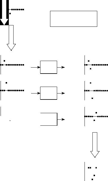
Any system with multiple inputs and/or outputs will be linear if it is composed of linear systems and signal additions.
Chapter 5- Linear Systems |
97 |
x1[n] |
System |
System |
y1[n] |
|
A |
B |
|
x2[n] |
System |
|
y2[n] |
|
C |
|
|
x3[n] |
System |
System |
y3[n] |
|
D |
E |
|
The use of multiplication in linear systems is frequently misunderstood. This is because multiplication can be either linear or nonlinear, depending on what the signal is multiplied by. Figure 5-9 illustrates the two cases. A system that multiplies the input signal by a constant, is linear. This system is an amplifier or an attenuator, depending if the constant is greater or less than one, respectively. In contrast, multiplying a signal by another signal is nonlinear. Imagine a sinusoid multiplied by another sinusoid of a different frequency; the resulting waveform is clearly not sinusoidal.
Another commonly misunderstood situation relates to parasitic signals added in electronics, such as DC offsets and thermal noise. Is the addition of these extraneous signals linear or nonlinear? The answer depends on where the contaminating signals are viewed as originating. If they are viewed as coming from within the system, the process is nonlinear. This is because a sinusoidal input does not produce a pure sinusoidal output. Conversely, the extraneous signal can be viewed as externally entering the system on a separate input of a multiple input system. This makes the process linear, since only a signal addition is required within the system.
x[n] |
x1[n] |
y[n] |
y[n] |
constant |
x2[n] |
Linear |
Nonlinear |
a. Multiplication by a constant |
b. Multiplication of two signals |
FIGURE 5-9
Linearity of multiplication. Multiplying a signal by a constant is a linear operation. In contrast, the multiplication of two signals is nonlinear.

98 |
The Scientist and Engineer's Guide to Digital Signal Processing |
Superposition: the Foundation of DSP
When we are dealing with linear systems, the only way signals can be combined is by scaling (multiplication of the signals by constants) followed by addition. For instance, a signal cannot be multiplied by another signal. Figure 5-10 shows an example: three signals: x0[n] , x1[n] , and x2[n] are added to form a fourth signal, x [n]. This process of combining signals through scaling and addition is called synthesis.
Decomposition is the inverse operation of synthesis, where a single signal is broken into two or more additive components. This is more involved than synthesis, because there are infinite possible decompositions for any given signal. For example, the numbers 15 and 25 can only be synthesized (added) into the number 40. In comparison, the number 40 can be decomposed into:
1 % 39 or 2 % 38 or & 30.5 % 60 % 10.5 , etc.
Now we come to the heart of DSP: superposition, the overall strategy for understanding how signals and systems can be analyzed. Consider an input
x0[n] 


 synthesis x[n]


decomposition
x1[n] 


FIGURE 5-10
Illustration of synthesis and decomposition of signals. In synthesis, two or more signals are added to form another signal. Decomposition is the opposite process, breaking one signal into two or more additive component signals.
x2[n] |
Chapter 5- Linear Systems |
99 |
x[n]
The Fundamental
Concept of DSP
decomposition
x0[n] |
System |
|
x1[n] |
System |
x2[n] 


 System
FIGURE 5-11
The fundamental concept in DSP. Any signal, such as x [n], can be decomposed into a group of additive components, shown here by the signals: x1[n], x2[n], and x3[n] . Passing these components through a linear system produces the signals, y1[n], y2[n], and y3[n] . The synthesis (addition) of these output signals forms y [n], the same signal produced when x [n] is passed through the system.
y0[n]
y1[n]
y2[n]
synthesis
y[n] 


signal, called x[n] , passing through a linear system, resulting in an output signal, y[n] . As illustrated in Fig. 5-11, the input signal can be decomposed into a group of simpler signals: x0[n] , x1[n] , x2[n] , etc. We will call these the input signal components. Next, each input signal component is individually passed through the system, resulting in a set of output signal components: y0[n] , y1[n] , y2[n] , etc. These output signal components are then synthesized into the output signal, y[n] .
100 |
The Scientist and Engineer's Guide to Digital Signal Processing |
Here is the important part: the output signal obtained by this method is identical to the one produced by directly passing the input signal through the system. This is a very powerful idea. Instead of trying to understanding how complicated signals are changed by a system, all we need to know is how simple signals are modified. In the jargon of signal processing, the input and output signals are viewed as a superposition (sum) of simpler waveforms. This is the basis of nearly all signal processing techniques.
As a simple example of how superposition is used, multiply the number 2041 by the number 4, in your head. How did you do it? You might have imagined 2041 match sticks floating in your mind, quadrupled the mental image, and started counting. Much more likely, you used superposition to simplify the problem. The number 2041 can be decomposed into: 2000 % 40 % 1 . Each of these components can be multiplied by 4 and then synthesized to find the final answer, i.e., 8000 % 160 % 4 ' 8164 .
Common Decompositions
Keep in mind that the goal of this method is to replace a complicated problem with several easy ones. If the decomposition doesn't simplify the situation in some way, then nothing has been gained. There are two main ways to decompose signals in signal processing: impulse decomposition and Fourier decomposition. They are described in detail in the next several chapters. In addition, several minor decompositions are occasionally used. Here are brief descriptions of the two major decompositions, along with three of the minor ones.
Impulse Decomposition
As shown in Fig. 5-12, impulse decomposition breaks an N samples signal into N component signals, each containing N samples. Each of the component signals contains one point from the original signal, with the remainder of the values being zero. A single nonzero point in a string of zeros is called an impulse. Impulse decomposition is important because it allows signals to be examined one sample at a time. Similarly, systems are characterized by how they respond to impulses. By knowing how a system responds to an impulse, the system's output can be calculated for any given input. This approach is called convolution, and is the topic of the next two chapters.
Step Decomposition
Step decomposition, shown in Fig. 5-13, also breaks an N sample signal into N component signals, each composed of N samples. Each component signal is a step, that is, the first samples have a value of zero, while the last samples are some constant value. Consider the decomposition of an N point signal, x[n] , into the components: x0[n], x1[n], x2[n], þxN& 1[n] . The k th component signal, xk[n] , is composed of zeros for points 0 through k& 1 , while the remaining points have a value of: x[k] & x[k& 1]. For example, the 5 th component signal, x5[n] , is composed of zeros for points 0 through 4, while the remaining samples have a value of: x[5] & x[4] (the difference between

Chapter 5- Linear Systems |
101 |
x[n] |
Impulse |
Decomposition |
x0[n] |
x1[n] |
x2[n] |
x27[n] |
FIGURE 5-12
Example of impulse decomposition. An N point signal is broken into N components, each consisting of a single nonzero point.
x[n] |
Step |
Decomposition |
x0[n]
x1[n] |
x2[n] |
x27[n] |
FIGURE 5-13
Example of step decomposition. An N point signal is broken into N signals, each consisting of a step function
sample 4 and 5 of the original signal). As a special case, x0[n] has all of its samples equal to x[0] . Just as impulse decomposition looks at signals one point at a time, step decomposition characterizes signals by the difference between adjacent samples. Likewise, systems are characterized by how they respond to a change in the input signal.

102 |
The Scientist and Engineer's Guide to Digital Signal Processing |
Even/Odd Decomposition
The even/odd decomposition, shown in Fig. 5-14, breaks a signal into two component signals, one having even symmetry and the other having odd symmetry. An N point signal is said to have even symmetry if it is a mirror image around point N/2 . That is, sample x[N/2 % 1] must equal x[N/2 & 1] , sample x[N/2 % 2] must equal x[N/2 & 2] , etc. Similarly, odd symmetry occurs when the matching points have equal magnitudes but are opposite in sign, such as: x[N/2 % 1] ' & x[N/2 & 1], x[N/2 % 2] ' & x[N/2 & 2], etc. These definitions assume that the signal is composed of an even number of samples, and that the indexes run from 0 to N& 1 . The decomposition is calculated from the relations:
EQUATION 5-1
Equations for even/odd decomposition. These equations separate a signal, x [n], into its even part, xE [n] , and its odd part, xO [n] . Since this decomposition is based on circularly symmetry, the zeroth samples in the even and odd signals are calculated: xE [0] ' x [0], and xO [0] ' 0 . All of the signals are N samples long, with indexes running from 0 to N-1
x |
|
[n ] ' |
x [n ] % x [N & n ] |
||
E |
|
||||
|
|
2 |
|||
|
|
|
|||
x |
|
|
[n ] ' |
x [n ] & x [N & n ] |
|
O |
|
|
|||
|
2 |
||||
|
|
|
|||
This may seem a strange definition of left-right symmetry, since N/2 & ½ (between two samples) is the exact center of the signal, not N/2 . Likewise, this off-center symmetry means that sample zero needs special handling. What's this all about?
This decomposition is part of an important concept in DSP called circular symmetry. It is based on viewing the end of the signal as connected to the beginning of the signal. Just as point x[4] is next to point x[5] , point x[N& 1] is next to point x[0] . Picture a snake biting its own tail. When even and odd signals are viewed in this circular manner, there are actually two lines of symmetry, one at point x[N/2] and another at point x[0] . For example, in an even signal, this symmetry around x[0] means that point x[1] equals point x[N& 1] , point x[2] equals point x[N& 2] , etc. In an odd signal, point 0 and point N/2 always have a value of zero. In an even signal, point 0 and point N /2 are equal to the corresponding points in the original signal.
What is the motivation for viewing the last sample in a signal as being next to the first sample? There is nothing in conventional data acquisition to support this circular notion. In fact, the first and last samples generally have less in common than any other two points in the sequence. It's common sense! The missing piece to this puzzle is a DSP technique called Fourier analysis. The mathematics of Fourier analysis inherently views the signal as being circular, although it usually has no physical meaning in terms of where the data came from. We will look at this in more detail in Chapter 10. For now, the important thing to understand is that Eq. 5-1 provides a valid decomposition, simply because the even and odd parts can be added together to reconstruct the original signal.

Chapter 5- Linear Systems |
103 |
x[n] |
Even/Odd
Decomposition
even symmetry |
xE[n] |
|
odd symmetry |
|
xO[n] |
|
|
0 |
N/2 |
N |
FIGURE 5-14
Example of even/odd decomposition. An N point signal is broken into two N point signals, one with even symmetry, and the other with odd symmetry.
x[n] |
Interlaced |
Decomposition |
even samples |
xE[n] |
odd samples |
xO[n] |
FIGURE 5-15
Example of interlaced decomposition. An N point signal is broken into two N point signals, one with the odd samples set to zero, the other with the even samples set to zero.
Interlaced Decomposition
As shown in Fig. 5-15, the interlaced decomposition breaks the signal into two component signals, the even sample signal and the odd sample signal (not to be confused with even and odd symmetry signals). To find the even sample signal, start with the original signal and set all of the odd numbered samples to zero. To find the odd sample signal, start with the original signal and set all of the even numbered samples to zero. It's that simple.
At first glance, this decomposition might seem trivial and uninteresting. This is ironic, because the interlaced decomposition is the basis for an extremely important algorithm in DSP, the Fast Fourier Transform (FFT). The procedure for calculating the Fourier decomposition has been known for several hundred years. Unfortunately, it is frustratingly slow, often requiring minutes or hours to execute on present day computers. The FFT is a family of algorithms developed in the 1960s to reduce this computation time. The strategy is an exquisite example of DSP: reduce the signal to elementary components by repeated use of the interlace transform; calculate the Fourier decomposition of the individual components; synthesize the results into the final answer. The
104 |
The Scientist and Engineer's Guide to Digital Signal Processing |
results are dramatic; it is common for the speed to be improved by a factor of hundreds or thousands.
Fourier Decomposition
Fourier decomposition is very mathematical and not at all obvious. Figure 5-16 shows an example of the technique. Any N point signal can be decomposed into N% 2 signals, half of them sine waves and half of them cosine waves. The lowest frequency cosine wave (called xC0 [n] in this illustration), makes zero complete cycles over the N samples, i.e., it is a DC signal. The next cosine components: xC1 [n], xC2 [n], and xC3 [n], make 1, 2, and 3 complete cycles over the N samples, respectively. This pattern holds for the remainder of the cosine waves, as well as for the sine wave components. Since the frequency of each component is fixed, the only thing that changes for different signals being decomposed is the amplitude of each of the sine and cosine waves.
Fourier decomposition is important for three reasons. First, a wide variety of signals are inherently created from superimposed sinusoids. Audio signals are a good example of this. Fourier decomposition provides a direct analysis of the information contained in these types of signals. Second, linear systems respond to sinusoids in a unique way: a sinusoidal input always results in a sinusoidal output. In this approach, systems are characterized by how they change the amplitude and phase of sinusoids passing through them. Since an input signal can be decomposed into sinusoids, knowing how a system will react to sinusoids allows the output of the system to be found. Third, the Fourier decomposition is the basis for a broad and powerful area of mathematics called Fourier analysis, and the even more advanced Laplace and z-transforms. Most cutting-edge DSP algorithms are based on some aspect of these techniques.
Why is it even possible to decompose an arbitrary signal into sine and cosine waves? How are the amplitudes of these sinusoids determined for a particular signal? What kinds of systems can be designed with this technique? These are the questions to be answered in later chapters. The details of the Fourier decomposition are too involved to be presented in this brief overview. For now, the important idea to understand is that when all of the component sinusoids are added together, the original signal is exactly reconstructed. Much more on this in Chapter 8.
Alternatives to Linearity
To appreciate the importance of linear systems, consider that there is only one major strategy for analyzing systems that are nonlinear. That strategy is to make the nonlinear system resemble a linear system. There are three common ways of doing this:
First, ignore the nonlinearity. If the nonlinearity is small enough, the system can be approximated as linear. Errors resulting from the original assumption are tolerated as noise or simply ignored.

Chapter 5- Linear Systems |
105 |
x[n]
Fourier
Decomposition
|
|
|
cosine waves |
|
|
|
|
sine waves |
|
|
|
|
|
|
|
|
|
|
|
|
|
|
|
|
|
|
|
|
|
|
|
|
|
|
|
|
|
||
xC0[n] |
|
|
|
xS0[n] |
|
|
|
||
|
|
|
|
|
|
|
|
|
|
xC1[n] |
xS1[n] |
xC2[n] |
xC3[n]
xS2[n] |
xS3[n] |
xC8[n] |
xS8[n] |
FIGURE 5-16
Illustration of Fourier decomposition. An N point signal is decomposed into N+2 signals, each having N points. Half of these signals are cosine waves, and half are sine waves. The frequencies of the sinusoids are fixed; only the amplitudes can change.
106 |
The Scientist and Engineer's Guide to Digital Signal Processing |
Second, keep the signals very small. Many nonlinear systems appear linear if the signals have a very small amplitude. For instance, transistors are very nonlinear over their full range of operation, but provide accurate linear amplification when the signals are kept under a few millivolts. Operational amplifiers take this idea to the extreme. By using very high open-loop gain together with negative feedback, the input signal to the op amp (i.e., the difference between the inverting and noninverting inputs) is kept to only a few microvolts. This minuscule input signal results in excellent linearity from an otherwise ghastly nonlinear circuit.
Third, apply a linearizing transform. For example, consider two signals being multiplied to make a third: a[n] ' b[n] × c[n]. Taking the logarithm of the signals changes the nonlinear process of multiplication into the linear process of addition: log( a[n]) ' log( b[n]) % log(c[n] ) . The fancy name for this approach is homomorphic signal processing. For example, a visual image can be modeled as the reflectivity of the scene (a two-dimensional signal) being multiplied by the ambient illumination (another two-dimensional signal). Homomorphic techniques enable the illumination signal to be made more uniform, thereby improving the image.
In the next chapters we examine the two main techniques of signal processing: convolution and Fourier analysis. Both are based on the strategy presented in this chapter: (1) decompose signals into simple additive components, (2) process the components in some useful manner, and (3) synthesize the components into a final result. This is DSP.