

Chapter 33The z-Transform |
615 |
simpler equations directly relating the pole-zero positions to the recursion coefficients. For example, a system containing two poles and two zeros, called as biquad, has the following relations:
EQUATION 33-5
Biquad design equations. These equations give the recursion coefficients, a0, a1, a2, b1, b2 , from the position of the poles: rp & Tp , and the zeros: r0 & T0 .
a0 |
' |
1 |
|
a1 |
' |
& 2 r0 cos (T0) |
|
a |
2 |
' |
r 2 |
|
|
0 |
|
b1 |
' |
2 rp cos(Tp ) |
|
b |
2 |
' |
& r 2 |
|
|
p |
|
After the transfer function has been specified, how do we find the frequency response? There are three methods: one is mathematical and two are computational (programming). The mathematical method is based on finding the values in the z-plane that lie on the unit circle. This is done by evaluating the transfer function, H (z ), at r ' 1 . Specifically, we start by writing down the transfer function in the form of either Eq. 33-3 or 33-4. We then replace each z with e & jT (that is, r e & jT with r ' 1 ). This provides a mathematical equation of the frequency response, H (T) . The problem is, the resulting expression is in a very inconvenient form. A significant amount of algebra is usually required to obtain something recognizable, such as the magnitude and phase. While this method provides an exact equation for the frequency response, it is difficult to automate in computer programs, such as needed in filter design packages.
The second method for finding the frequency response also uses the approach of evaluating the z-plane on the unit circle. The difference is that we only calculate samples of the frequency response, not a mathematical solution for the entire curve. A computer program loops through, perhaps, 1000 equally spaced frequencies between T' 0 and T' B. Think of an ant moving between 1000 discrete points on the upper half of the z-plane's unit circle. The magnitude and phase of the frequency response are found at each of these location by evaluating the transfer function.
This method works well and is often used in filter design packages. Its major limitation is that it does not account for round-off noise affecting the system's characteristics. Even if the frequency response found by this method looks perfect, the implemented system can be completely unstable!
This brings up the third method: find the frequency response from the recursion coefficients that are actually used to implement the filter. To start, we find the impulse response of the filter by passing an impulse through the system. In the second step, we take the DFT of the impulse response (using the FFT, of course) to find the system's frequency response. The only critical item to remember with this procedure is that enough samples must be taken of the impulse response so that the discarded samples are insignificant. While books

616 |
The Scientist and Engineer's Guide to Digital Signal Processing |
could be written on the theoretical criteria for this, the practical rules are much simpler. Use as many samples as you think are necessary. After finding the frequency response, go back and repeat the procedure using twice as many samples. If the two frequency responses are adequately similar, you can be assured that the truncation of the impulse response hasn't fooled you in some way.
Cascade and Parallel Stages
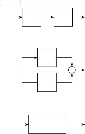
Sophisticated recursive filters are usually designed in stages to simplify the tedious algebra of the z-domain. Figure 33-4 illustrates the two common ways that individual stages can be arranged: cascaded stages and parallel stages with added outputs. For example, a low-pass and high-pass stage can be cascaded to form a band-pass filter. Likewise, a parallel combination of low-pass and high-pass stages can form a band-reject filter. We will call the two stages being combined system 1 and system 2, with their recursion coefficients being called: a0, a1, a2, b1, b2 and A0, A1, A2, B1, B2 , respectively. Our goal is to combine these stages (in cascade or parallel) into a single recursive filter, which we will call system 3, with recursion coefficients given by: a0, a1, a2, a3, a4, b1, b2, b3, b4 .
As you recall from previous chapters, the frequency responses of systems in a cascade are combined by multiplication. Also, the frequency responses of systems in parallel are combined by addition. These same rules are followed by the z-domain transfer functions. This allows recursive systems to be combined by moving the problem into the z-domain, performing the required multiplication or addition, and then returning to the recursion coefficients of the final system.
As an example of this method, we will work out the algebra for combining two biquad stages in a cascade. The transfer function of each stage is found by writing Eq. 33-3 using the appropriate recursion coefficients. The transfer function of the entire system, H [z ] , is then found by multiplying the transfer functions of the two stage:
|
a |
0 |
% a |
|
z & 1 % a |
|
z & 2 |
|
A |
0 |
% A |
|
z & 1 % A |
|
z & 2 |
|||||
H [z ] ' |
|
1 |
|
|
2 |
|
× |
|
1 |
|
|
2 |
|
|||||||
1 & b |
z & 1 |
& b |
2 |
z & 2 |
1 & B |
z & 1 |
& B |
2 |
z & 2 |
|||||||||||
|
|
|||||||||||||||||||
|
|
|
1 |
|
|
|
|
|
|
|
|
1 |
|
|
|
|
|
|||
Multiplying out the polynomials and collecting like terms:
|
a |
A |
0 |
% (a |
A |
% a |
A |
) z & 1 % (a |
A |
% a |
A |
% a |
A |
) z & 2 % (a |
A |
% a |
A |
) z & 3 % (a |
A |
) z & 4 |
||||||||||||
H [z ] ' |
0 |
|
0 |
|
1 |
|
1 |
0 |
|
|
0 |
|
2 |
|
1 |
|
1 |
2 |
0 |
|
|
1 |
2 |
2 |
1 |
|
|
2 |
2 |
|
|
|
|
|
|
1 & (b |
% B |
) z & 1 |
& (b |
% B |
& b |
B |
) z & 2 & (& b |
B |
& b |
B |
) z & 3 & (& b |
B |
) z & 4 |
|
|
||||||||||||||
|
|
|
|
|
|
|||||||||||||||||||||||||||
|
|
|
|
|
1 |
|
1 |
|
|
|
2 |
|
2 |
|
1 |
|
1 |
|
|
|
1 |
2 |
2 |
1 |
|
|
2 |
2 |
|
|
|
|
Chapter 33The z-Transform |
617 |
a. Cascade
FIGURE 33-4
Combining cascade and parallel stages. The z-domain allows recursive stages in a cascade, (a), or in parallel, (b), to be combined into a single system, (c).
|
|
System 1 |
|
System 2 |
||
x[n] |
|
|
y[n] |
|||
|
|
a0, a1, a2 |
|
A0, A1, A2 |
|
|
|
|
|
|
|||
|
|
b1, b2 |
|
B1, B2 |
||
b. Parallel |
|
System 1 |
||||||
|
|
|
a0, a1, a2 |
|||||
x[n] |
b1, b2 |
|||||||
|
|
|
|
y[n] |
||||
|
|
|
|
|
|
|
|
|
|
|
|
|
|
|
|
|
|
System 2
 A0, A1, A2
B1, B2
c. Replacement |
|
|
|
|
x[n] |
System 3 |
|||
a0, a1, a2, a3, a4 |
y[n] |
|||
|
|
|
|
|
|
|
|
||
|
|
b1, b2, b3, b4 |
||
Since this is in the form of Eq. 33-3, we can directly extract the recursion coefficients that implement the cascaded system:
a0 |
' |
a0 A0 |
|
|
a1 ' a0 A1 % a1 A0 |
b1 |
' b1 % B1 |
||
a2 |
' a0 A2 % a1 A1 % a2 A0 |
b2 |
' b2 % B2 & b1 B1 |
|
a3 |
' a1 A2 % a2 A1 |
b3 |
' & b1 B2 & b2 B1 |
|
a4 |
' a2 A2 |
b4 |
' & b2 B2 |
|
The obvious problem with this technique is the large amount of algebra needed to multiply and rearrange the polynomial terms. Fortunately, the entire algorithm can be expressed in a short computer program, shown in Table 33-1. Although the cascade and parallel combinations require different mathematics, they use nearly the same program. In particular, only one line of code is different between the two algorithms, allowing both to be combined into a single program.
618 |
The Scientist and Engineer's Guide to Digital Signal Processing |
|
100 'COMBINING RECURSION COEFFICIENTS OF CASCADE AND PARALLEL STAGES |
||
110 ' |
|
|
120 ' |
'INITIALIZE VARIABLES |
|
130 |
DIM A1[8], B1[8] |
'a and b coefficients for system 1, one of the stages |
140 |
DIM A2[8], B2[8] |
'a and b coefficients for system 2, one of the stages |
150 |
DIM A3[16], B3[16] |
'a and b coefficients for system 3, the combined system |
160 ' |
|
|
170 |
|
'Indicate cascade or parallel combination |
180 |
INPUT "Enter 0 for cascade, 1 for parallel: ", CP% |
|
190 ' |
|
|
200 |
GOSUB XXXX |
'Mythical subroutine to load: A1[ ], B1[ ], A2[ ], B2[ ] |
210 ' |
|
|
220 |
FOR I% = 0 TO 8 |
'Convert the recursion coefficients into transfer functions |
230 |
B2[I%] = -B2[I%] |
|
240 |
B1[I%] = -B1[I%] |
|
250 NEXT I% |
|
|
260 |
B1[0] = 1 |
|
270 |
B2[0] = 1 |
|
280 ' |
|
|
290 |
FOR I% = 0 TO 16 |
'Multiply the polynomials by convolving |
300 |
A3[I%] = 0 |
|
310 |
B3[I%] = 0 |
|
320 |
FOR J% = 0 TO 8 |
|
330 |
IF I%-J% < 0 OR I%-J% > 8 THEN GOTO 370 |
|
340 |
IF CP% = 0 THEN A3[I%] = A3[I%] + A1[J%] * A2[I%-J%] |
|
350 |
IF CP% = 1 THEN A3[I%] = A3[I%] + A1[J%] * B2[I%-J%] + A2[J%] * B1[I%-J%] |
|
360 |
B3[I%] = B3[I%] + B1[J%] * B2[I%-J%] |
|
370 |
NEXT J% |
|
380 NEXT I% |
|
|
390 ' |
|
|
400 |
FOR I% = 0 TO 16 |
'Convert the transfer function into recursion coefficients. |
410 |
B3[I%] = -B3[I%] |
|
420 NEXT I% |
|
|
430 |
B3[0] = 0 |
|
440 ' |
'The recursion coefficients of the combined system now |
|
450 |
END |
'reside in A3[ ] & B3[ ] |
TABLE 33-1
Combining cascade and parallel stages. This program combines the recursion coefficients of stages in cascade or parallel. The recursive coefficients for the two stages being combined enter the program in the arrays: A1[ ], B1[ ], & A2[ ], B2[ ]. The recursion coefficients that implement the entire system leave the program in the arrays: A3[ ], B3[ ].
This program operates by changing the recursive coefficients from each of the individual stages into transfer functions in the form of Eq. 33-3 (lines 220270). After combining these transfer functions in the appropriate manner (lines 290-380), the information is moved back to being recursive coefficients (lines 400 to 430).
The heart of this program is how the transfer function polynomials are represented and combined. For example, the numerator of the first stage being combined is: a0 % a1 z & 1 % a2 z & 2 % a3 z & 3 þ . This polynomial is represented in the program by storing the coefficients: a0, a1, a2, a3 þ , in the array: A1[0], A1[1], A1[2], A1[3]þ . Likewise, the numerator for the second stage is represented by the values stored in: A2[0], A2[1], A2[2], A2[3]þ, and the numerator for the combined system in: A3[0], A3[1], A3[2], A3[3]þ. The
Chapter 33The z-Transform |
619 |
idea is to represent and manipulate polynomials by only referring to their coefficients. The question is, how do we calculate A3[ ], given that A1[ ], A2[ ], and A3[ ] all represent polynomials? The answer is that when two polynomials are multiplied, their coefficients are convolved. In equation form: A1[ ] ( A2[ ] ' A3[ ] . This allows a standard convolution algorithm to find the transfer function of cascaded stages by convolving the two numerator arrays and the two denominator arrays.
The procedure for combining parallel stages is slightly more complicated. In algebra, fractions are added according to:
w |
% |
y |
' |
w@z % x @y |
|
|
x @z |
||
x z |
||||
Since each of the transfer functions is a fraction (one polynomial divided by another polynomial), we combine stages in parallel by multiplying the denominators, and adding the cross products in the numerators. This means that the denominator is calculated in the same way as for cascaded stages, but the numerator calculation is more elaborate. In line 340, the numerators of cascaded stages are convolved to find the numerator of the combined transfer function. In line 350, the numerator of the p a r a l l e l stage combination is calculated as the sum of the two numerators convolved with the two denominators. Line 360 handles the denominator calculation for both cases.
Spectral Inversion
Chapter 14 describes an FIR filter technique called spectral inversion. This is a way of changing the filter kernel such that the frequency response is flipped top-for-bottom. All the passbands are changed into stopbands, and vice versa. For example, a low-pass filter is changed into high-pass, a band-pass filter into band-reject, etc. A similar procedure can be done with recursive filters, although it is far less successful.
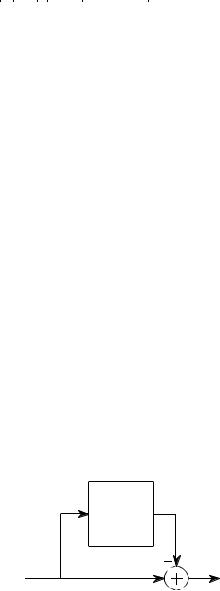
As illustrated in Fig. 33-5, spectral inversion is accomplished by subtracting the output of the system from the original signal. This procedure can be
FIGURE 33-5
Spectral inversion. This procedure is the same as subtracting the output of the system from the original signal.
Original
System
x[n] |
y[n] |
620 |
The Scientist and Engineer's Guide to Digital Signal Processing |
viewed as combining two stages in parallel, where one of the stages happens to be the identity system (the output is identical to the input). Using this approach, it can be shown that the "b" coefficients are left unchanged, and the modified "a" coefficients are given by:
EQUATION 33-6
Spectral inversion. The frequency response of a recursive filter can be flipped top-for- bottom by modifying the "a" coefficients according to these equations. The original coefficients are shown in italics, and the modified coefficients in roman. The "b" coefficients are not changed. This method usually provides poor results.
a0 ' 1 & a0
a1 ' & a1 & b1 a2 ' & a2 & b2 a3 ' & a3 & b3
!
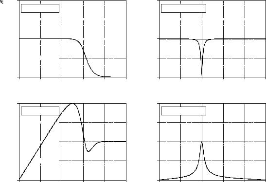
Figure 33-6 shows spectral inversion for two common frequency responses: a low-pass filter, (a), and a notch filter, (c). This results in a high-pass filter, (b), and a band-pass filter, (d), respectively. How do the resulting frequency responses look? The high-pass filter is absolutely terrible! While
Amplitude
Amplitude
2.0
a. Original LP
1.5 


1.0 


0.5 


0.0
0 0.1 0.2 0.3 0.4 0.5
Frequency
2.0
b. Inverted LP
1.5 


1.0 


0.5 


0.0
0 0.1 0.2 0.3 0.4 0.5
Frequency
2.0
c. Original notch
1.5 


Amplitude |
1.0 |
|
|
|
|
|
|
|
|
|
|
|
|
|
0.5 |
|
|
|
|
|
|
0.0 |
|
|
|
|
|
|
0 |
0.1 |
0.2 |
0.3 |
0.4 |
0.5 |
|
|
|
Frequency |
|
|
|
|
2.0 |
|
|
|
|
|
|
|
d. Inverted notch |
|
|
|
|
|
1.5 |
|
|
|
|
|
Amplitude |
|
|
|
|
|
|
Amplitude |
1.0 |
|
|
|
|
|
|
|
|
|
|
|
|
|
0.5 |
|
|
|
|
|
|
0.0 |
|
|
|
|
|
|
0 |
0.1 |
0.2 |
0.3 |
0.4 |
0.5 |
Frequency
FIGURE 33-6
Examples of spectral inversion. Figure (a) shows the frequency response of a 6 pole low-pass Butterworth filter. Figure (b) shows the corresponding high-pass filter obtained by spectral inversion; its a mess! A more successful case is shown in (c) and (d) where a notch filter is transformed in to a band-pass frequency response.

Chapter 33The z-Transform |
621 |
the band-pass is better, the peak is not as sharp as the notch filter from which it was derived. These mediocre results are especially disappointing in comparison to the excellent performance seen in Chapter 14. Why the difference? The answer lies in something that is often forgotten in filter design: the phase response.
To illustrate how phase is the culprit, consider a system called the Hilbert transformer. The Hilbert transformer is not a specific device, but any system that has the frequency response: Magnitude = 1 and phase = 90 degrees, for all frequencies. This means that any sinusoid passing through a Hilbert transformer will be unaffected in amplitude, but changed in phase by onequarter of a cycle. Hilbert transformers can be analog or discrete (that is, hardware or software), and are commonly used in communications for various modulation and demodulation techniques.
Now, suppose we spectrally invert the Hilbert transformer by subtracting its output from the original signal. Looking only at the magnitude of the frequency responses, we would conclude that the entire system would have an output of zero. That is, the magnitude of the Hilbert transformer's output is identical to the magnitude of the original signal, and the two will cancel. This, of course, is completely incorrect. Two sinusoids will exactly cancel only if they have the same magnitude and phase. In reality, the frequency response of this composite system has a magnitude of  2 , and a phase shift of -45 degrees. Rather than being zero (our naive guess), the output is larger in amplitude than the input!
Spectral inversion works well in Chapter 14 because of the specific kind of filter used: zero phase. That is, the filter kernels have a left-right symmetry. When there is no phase shift introduced by a system, the subtraction of the output from the input is dictated solely by the magnitudes. Since recursive filters are plagued with phase shift, spectral inversion generally produces unsatisfactory filters.
Gain Changes
Suppose we have a recursive filter and need to modify the recursion coefficients such that the output signal is changed in amplitude. This might be needed, for example, to insure that a filter has unity gain in the passband. The method to achieve this is very simple: multiply the "a" coefficients by whatever factor we want the gain to change by, and leave the "b" coefficients alone.
Before adjusting the gain, we would probably like to know its current value. Since the gain must be specified at a frequency in the passband, the procedure depends on the type of filter being used. Low-pass filters have their gain measured at a frequency of zero, while high-pass filters use a frequency of 0.5, the maximum frequency allowable. It is quite simple to derive expressions for the gain at both these special frequencies. Here's how it is done.

622 |
The Scientist and Engineer's Guide to Digital Signal Processing |
First, we will derive an equation for the gain at zero frequency. The idea is to force each of the input samples to have a value of one, resulting in each of the output samples having a value of G, the gain of the system we are trying to find. We will start by writing the recursion equation, the mathematical relationship between the input and output signals:
y [n ] ' a0 x [n ] % a1 x [n & 1] % a2 x [n & 2] % þ% b1 y [n & 1] % b2 y [n & 2] % b3 y [n & 3] % þ
Next, we plug in one for each input sample, and G for each output sample. In other words, we force the system to operate at zero frequency. The equation becomes:
G ' a0 % a1 % a2 % a3 % þ % b1 G % b2 G % b3 G % b4 G þ
Solving for G provides the gain of the system at zero frequency, based on its recursion coefficients:
EQUATION 33-7
DC gain of recursive filters. This relation provides the DC gain from the recursion coefficients.
G ' a0 % a1 % a2 % a3þ
1 & (b1 % b2 % b3þ)
To make a filter have a gain of one at DC, calculate the existing gain by using this relation, and then divide all the "a" coefficients by G.
The gain at a frequency of 0.5 is found in a similar way: we force the input and output signals to operate at this frequency, and see how the system responds. At a frequency of 0.5, the samples in the input signal alternate between -1 and 1. That is, successive samples are: 1, -1, 1, -1, 1, -1, 1, etc. The corresponding output signal also alternates in sign, with an amplitude equal to the gain of the system: G, -G, G, -G, G, -G, etc. Plugging these signals into the recursion equation:
G ' a0 & a1 % a2 & a3 % þ & b1 G % b2 G & b3 G % b4 G þ
Solving for G provides the gain of the system at a frequency of 0.5, using its recursion coefficients:
EQUATION 33-8
Gain at maximum frequency. This relation gives the recursive filter's gain at a frequency of 0.5, based on the system's recursion coefficients.
G ' a0 & a1 % a2 & a3 % a4 þ 1 & (& b1 % b2 & b3 % b4 þ)
Chapter 33The z-Transform |
623 |
Just as before, a filter can be normalized for unity gain by dividing all of the "a" coefficients by this calculated value of G. Calculation of Eq. 33-8 in a computer program requires a method for generating negative signs for the odd coefficients, and positive signs for the even coefficients. The most common method is to multiply each coefficient by (&1)k , where k is the index of the coefficient being worked on. That is, as k runs through the values: 0, 1, 2, 3, 4, 5, 6 etc., the expression, (&1)k , takes on the values: 1, -1, 1, -1, 1, -1, 1 etc.
Chebyshev-Butterworth Filter Design
A common method of designing recursive digital filters is shown by the Chebyshev-Butterworth program presented in Chapter 20. It starts with a polezero diagram of an analog filter in the s-plane, and converts it into the desired digital filter through several mathematical transforms. To reduce the complexity of the algebra, the filter is designed as a cascade of several stages, with each stage implementing one pair of poles. The recursive coefficients for each stage are then combined into the recursive coefficients for the entire filter. This is a very sophisticated and complicated algorithm; a fitting way to end this book. Here's how it works.
Loop Control
Figure 33-7 shows the program and flowchart for the method, duplicated from Chapter 20. After initialization and parameter entry, the main portion of the program is a loop that runs through each pole-pair in the filter. This loop is controlled by block 11 in the flowchart, and the FOR-NEXT loop in lines 320 & 460 of the program. For example, the loop will be executed three times for a 6 pole filter, with the loop index, P%, taking on the values 1,2,3. That is, a 6 pole filter is implemented in three stages, with two poles per stage.
Combining Coefficients
During each loop, subroutine 1000 (listed in Fig. 33-8) calculates the recursive coefficients for that stage. These are returned from the subroutine in the five variables: A0, A1, A2, B1, B2 . In step 10 of the flowchart (lines 360-440), these coefficients are combined with the coefficients of all the previous stages, held in the arrays: A[ ] and B[ ]. At the end of the first loop, A[ ] and B[ ] hold the coefficients for stage one. At the end of the second loop, A[ ] and B[ ] hold the coefficients of the cascade of stage one and stage two. When all the loops have been completed, A[ ] and B[ ] hold the coefficients needed to implement the entire filter.
The coefficients are combined as previously outlined in Table 33-1, with a few modifications to make the code more compact. First, the index of the arrays, A[ ] and B[ ], is shifted by two during the loop. For example, a0 is held in A[2], a1 & b1 are held in A[3] & B[3], etc. This is done to prevent the program from trying to access values outside the defined arrays. This shift is removed in block 12 (lines 480-520), such that the final recursion coefficients reside in A[ ] and B[ ] without an index offset.
624 |
The Scientist and Engineer's Guide to Digital Signal Processing |
Second, A[ ] and B[ ] must be initialized with coefficients corresponding to the identity system, not all zeros. This is done in lines 180 to 240. During the first loop, the coefficients for the first stage are combined with the information initially present in these arrays. If all zeros were initially present, the arrays would always remain zero. Third, two temporary arrays are used, TA[ ] and TB[ ]. These hold the old values of A[ ] and B[ ] during the convolution, freeing A[ ] and B[ ] to hold the new values.
To finish the program, block 13 (lines 540-670) adjusts the filter to have a unity gain in the passband. This operates as previously described: calculate the existing gain with Eq. 33-7 or 33-8, and divide all the "a" coefficients to normalize. The intermediate variables, SA and SB, are the sums of the "a" and "b" coefficients, respectively.
Calculate Pole Locations in the s-Plane
Regardless of the type of filter being designed, this program begins with a Butterworth low-pass filter in the s-plane, with a cutoff frequency of T ' 1 . As described in the last chapter, Butterworth filters have poles that are equally spaced around a circle in the s-plane. Since the filter is low-pass, no zeros are used. The radius of the circle is one, corresponding to the cutoff frequency of T ' 1 . Block 3 of the flowchart (lines 1080 & 1090) calculate the location of each pole-pair in rectangular coordinates. The program variables, RP and IP, are the real and imaginary parts of the pole location, respectively. These program variables correspond to F and T, where the pole-pair is located at F ± jT. This pole location is calculated from the number of poles in the filter and the stage being worked on, the program variables: NP and P%, respectively.
Warp from Circle to Ellipse
To implement a Chebyshev filter, this circular pattern of poles must be transformed into an elliptical pattern. The relative flatness of the ellipse determines how much ripple will be present in the passband of the filter. If the pole location on the circle is given by: F and T, the corresponding location on the ellipse, Fr and Tr, is given by:
EQUATION 33-9
Circular to elliptical transform. These equations change the pole location on a circle to a corresponding location on an ellipse. The variables, NP and PR, are the number of poles in the filter, and the p e r c e n t r i p p l e i n t h e p a s s b a n d , respectively. The location on the circle is given by F and T, and the location on the ellipse by F3 and T3. The variables ,, v, and k, are used only to make the equations shorter.
Fr ' F sinh(v) / k
Tr ' T cosh (v) / k
where: |
' |
sinh& 1 |
(1/,) |
|
|
v |
NP |
|
|
|
|
|
|
|
|
|
|
k |
' cosh |
1 cosh& 1 1 |
|||
|
|
NP |
|
, |
|
, ' |
100 |
2 |
1/2 |
||
|
& 1 |
||||
100 & PR |
|
||||
|
|
|
|
||