

CHAPTER
ADC and DAC
3
Most of the signals directly encountered in science and engineering are continuous: light intensity that changes with distance; voltage that varies over time; a chemical reaction rate that depends on temperature, etc. Analog-to-Digital Conversion (ADC) and Digital-to-Analog Conversion (DAC) are the processes that allow digital computers to interact with these everyday signals. Digital information is different from its continuous counterpart in two important respects: it is sampled, and it is quantized. Both of these restrict how much information a digital signal can contain. This chapter is about information management: understanding what information you need to retain, and what information you can afford to lose. In turn, this dictates the selection of the sampling frequency, number of bits, and type of analog filtering needed for converting between the analog and digital realms.
Quantization
First, a bit of trivia. As you know, it is a digital computer, not a digit computer. The information processed is called digital data, not digit data. Why then, is analog-to-digital conversion generally called: digitize and digitization, rather than digitalize and digitalization? The answer is nothing you would expect. When electronics got around to inventing digital techniques, the preferred names had already been snatched up by the medical community nearly a century before. Digitalize and digitalization mean to administer the heart stimulant digitalis.
Figure 3-1 shows the electronic waveforms of a typical analog-to-digital conversion. Figure (a) is the analog signal to be digitized. As shown by the labels on the graph, this signal is a voltage that varies over time. To make the numbers easier, we will assume that the voltage can vary from 0 to 4.095 volts, corresponding to the digital numbers between 0 and 4095 that will be produced by a 12 bit digitizer. Notice that the block diagram is broken into two sections, the sample-and-hold (S/H), and the analog-to-digital converter (ADC). As you probably learned in electronics classes, the sample-and-hold is required to keep the voltage entering the ADC constant while the
35

36 |
The Scientist and Engineer's Guide to Digital Signal Processing |
conversion is taking place. However, this is not the reason it is shown here; breaking the digitization into these two stages is an important theoretical model for understanding digitization. The fact that it happens to look like common electronics is just a fortunate bonus.
As shown by the difference between (a) and (b), the output of the sample-and- hold is allowed to change only at periodic intervals, at which time it is made identical to the instantaneous value of the input signal. Changes in the input signal that occur between these sampling times are completely ignored. That is, sampling converts the independent variable (time in this example) from continuous to discrete.
As shown by the difference between (b) and (c), the ADC produces an integer value between 0 and 4095 for each of the flat regions in (b). This introduces an error, since each plateau can be any voltage between 0 and 4.095 volts. For example, both 2.56000 volts and 2.56001 volts will be converted into digital number 2560. In other words, quantization converts the dependent variable (voltage in this example) from continuous to discrete.
Notice that we carefully avoid comparing (a) and (c), as this would lump the sampling and quantization together. It is important that we analyze them separately because they degrade the signal in different ways, as well as being controlled by different parameters in the electronics. There are also cases where one is used without the other. For instance, sampling without quantization is used in switched capacitor filters.
First we will look at the effects of quantization. Any one sample in the digitized signal can have a maximum error of ±½ LSB (Least Significant Bit, jargon for the distance between adjacent quantization levels). Figure (d) shows the quantization error for this particular example, found by subtracting
(b) from (c), with the appropriate conversions. In other words, the digital output (c), is equivalent to the continuous input (b), plus a quantization error
(d). An important feature of this analysis is that the quantization error appears very much like random noise.
This sets the stage for an important model of quantization error. In most cases, quantization results in nothing more than the addition of a specific amount of random noise to the signal. The additive noise is uniformly distributed between ±½ LSB, has a mean of zero, and a standard deviation of 1/ 12 LSB (-0.29 LSB). For example, passing an analog signal through an 8 bit digitizer adds an rms noise of: 0.29 /256 , or about 1/900 of the full scale value. A 12 bit conversion adds a noise of: 0.29 /4096 . 1 /14,000 , while a 16 bit conversion adds: 0.29 /65536 . 1 /227,000 . Since quantization error is a random noise, the number of bits determines the precision of the data. For example, you might make the statement: "We increased the precision of the measurement from 8 to 12 bits."
This model is extremely powerful, because the random noise generated by quantization will simply add to whatever noise is already present in the

Chapter 3- ADC and DAC |
37 |
|
3.025 |
|
|
|
|
|
|
|
|
|
|
|
|
a. Original analog signal |
|
|
|
|
|||||
volts) |
3.020 |
|
|
|
|
|
|
|
|
|
|
3.015 |
|
|
|
|
|
|
|
|
|
|
|
(in |
|
|
|
|
|
|
|
|
|
|
|
|
|
|
|
|
|
|
|
|
|
|
|
Amplitude |
3.010 |
|
|
|
|
|
|
|
|
|
|
|
|
|
|
|
|
|
|
|
|
|
|
|
3.005 |
|
|
|
|
|
|
|
|
|
|
|
3.000 |
|
|
|
|
|
|
|
|
|
|
|
0 |
5 |
10 |
15 |
20 |
25 |
30 |
35 |
40 |
45 |
50 |
|
|
|
|
|
|
Time |
|
|
|
|
|
FIGURE 3-1
Waveforms illustrating the digitization process. The conversion is broken into two stages to allow the effects of sampling to be separated from the effects of quantization. The first stage is the sample-and-hold (S/H), where the only information retained is the instantaneous value of the signal when the periodic sampling takes place. In the second stage, the ADC converts the voltage to the nearest integer number. This results in each sample in the digitized signal having an error of up to ±½ LSB, as shown in (d). As a result, quantization can usually be modeled as simply adding noise to the signal.
analog |
digital |
input |
output |
S/H 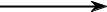 ADC
ADC
Amplitude (in volts)
3.025 |
|
|
|
|
|
|
|
|
|
|
|
b. Sampled analog signal |
|
|
|
|
|||||
3.020 |
|
|
|
|
|
|
|
|
|
|
3.015 |
|
|
|
|
|
|
|
|
|
|
3.010 |
|
|
|
|
|
|
|
|
|
|
3.005 |
|
|
|
|
|
|
|
|
|
|
3.000 |
|
|
|
|
|
|
|
|
|
|
0 |
5 |
10 |
15 |
20 |
25 |
30 |
35 |
40 |
45 |
50 |
|
|
|
|
|
Time |
|
|
|
|
|
Digital number
3025
c. Digitized signal
3020
3015 

3010
3005
3000
0 |
5 |
10 |
15 |
20 |
25 |
30 |
35 |
40 |
45 |
50 |
Sample number
Error (in LSBs)
1.0
d. Quantization error |
0.5
0.0
-0.5
-1.0
0 |
5 |
10 |
15 |
20 |
25 |
30 |
35 |
40 |
45 |
50 |
Sample number

38 |
The Scientist and Engineer's Guide to Digital Signal Processing |
analog signal. For example, imagine an analog signal with a maximum amplitude of 1.0 volt, and a random noise of 1.0 millivolt rms. Digitizing this signal to 8 bits results in 1.0 volt becoming digital number 255, and 1.0 millivolt becoming 0.255 LSB. As discussed in the last chapter, random noise signals are combined by adding their variances. That is, the signals are added in quadrature:  A 2 %B 2 ' C . The total noise on the digitized signal is therefore given by:
  0.2552 % 0.292 ' 0.386 LSB. This is an increase of about 50% over the noise already in the analog signal. Digitizing this same signal to 12 bits would produce virtually no increase in the noise, and nothing would be lost due to quantization. When faced with the decision of how many bits are needed in a system, ask two questions: (1) How much noise is already present in the analog signal? (2) How much noise can be tolerated in the digital signal?
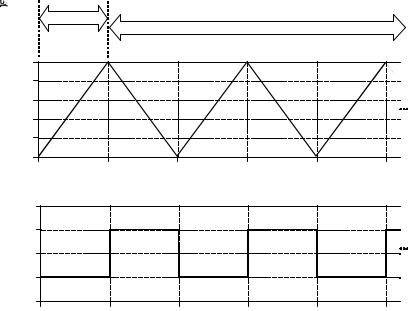
When isn't this model of quantization valid? Only when the quantization error cannot be treated as random. The only common occurrence of this is when the analog signal remains at about the same value for many consecutive samples, as is illustrated in Fig. 3-2a. The output remains stuck on the same digital number for many samples in a row, even though the analog signal may be changing up to ±½ LSB. Instead of being an additive random noise, the quantization error now looks like a thresholding effect or weird distortion.
Dithering is a common technique for improving the digitization of these slowly varying signals. As shown in Fig. 3-2b, a small amount of random noise is added to the analog signal. In this example, the added noise is normally distributed with a standard deviation of 2/3 LSB, resulting in a peak- to-peak amplitude of about 3 LSB. Figure (c) shows how the addition of this dithering noise has affected the digitized signal. Even when the original analog signal is changing by less than ±½ LSB, the added noise causes the digital output to randomly toggle between adjacent levels.
To understand how this improves the situation, imagine that the input signal is a constant analog voltage of 3.0001 volts, making it one-tenth of the way between the digital levels 3000 and 3001. Without dithering, taking 10,000 samples of this signal would produce 10,000 identical numbers, all having the value of 3000. Next, repeat the thought experiment with a small amount of dithering noise added. The 10,000 values will now oscillate between two (or more) levels, with about 90% having a value of 3000, and 10% having a value of 3001. Taking the average of all 10,000 values results in something close to 3000.1. Even though a single measurement has the inherent ±½ LSB limitation, the statistics of a large number of the samples can do much better. This is quite a strange situation: adding noise provides more information.
Circuits for dithering can be quite sophisticated, such as using a computer to generate random numbers, and then passing them through a DAC to produce the added noise. After digitization, the computer can subtract
Chapter 3- ADC and DAC |
39 |
|
3005 |
|
|
|
|
|
|
|
|
|
|
number) |
|
a. Digitization of a small amplitude signal |
|
||||||||
3004 |
|
|
|
|
|
|
|
|
|
|
|
digital(or |
|
|
|
|
|
|
|
|
|
|
|
3002 |
|
|
|
analog signal |
|
|
|
|
|||
|
3003 |
|
|
|
|
|
|
|
|||
Millivolts |
3001 |
|
|
|
|
|
|
|
|
|
|
|
|
|
|
|
|
|
|
|
|
|
|
|
3000 |
|
|
|
|
digital signal |
|
|
|
||
|
|
|
|
|
|
|
|
|
|
|
|
|
0 |
5 |
10 |
15 |
20 |
25 |
30 |
35 |
40 |
45 |
50 |
Time (or sample number)
FIGURE 3-2
Illustration of dithering. Figure (a) shows how an analog signal that varies less than ±½ LSB can become stuck on the same quantization level during digitization. Dithering improves this situation by adding a small amount of random noise to the analog signal, such as shown in (b). In this example, the added noise is normally distributed with a standard deviation of 2/3 LSB. As shown in (c), the added noise causes the digitized signal to toggle between adjacent quantization levels, providing more information about the original signal.
3005
b. Dithering noise added
3004
original analog signal
Millivolts |
3003 |
3002 |
|
|
3001 |

 with added noise
|
3000 |
|
|
|
|
|
|
|
|
|
|
|
0 |
5 |
10 |
15 |
20 |
25 |
30 |
35 |
40 |
45 |
50 |
|
|
|
|
|
|
Time |
|
|
|
|
|
|
3005 |
|
|
|
|
|
|
|
|
|
|
number) |
|
c. Digitization of dithered signal |
|
|
|
||||||
3004 |
|
|
|
|
|
|
|
|
|
|
|
|
|
original analog signal |
|
|
|
|
|
||||
|
|
|
|
|
|
|
|
|
|
|
|
(or digital |
3003 |
|
|
|
|
|
|
|
|
|
|
3002 |
|
|
|
|
|
|
|
|
|
|
|
Millivolts |
3001 |
|
|
|
|
|
|
|
|
|
|
|
|
|
|
|
|
|
|
|
|
|
|
|
3000 |
|
|
|
|
digital signal |
|
|
|
||
|
|
|
|
|
|
|
|
|
|
|
|
|
0 |
5 |
10 |
15 |
20 |
25 |
30 |
35 |
40 |
45 |
50 |
Time (or sample number)
the random numbers from the digital signal using floating point arithmetic. This elegant technique is called subtractive dither, but is only used in the most elaborate systems. The simplest method, although not always possible, is to use the noise already present in the analog signal for dithering.
The Sampling Theorem
The definition of proper sampling is quite simple. Suppose you sample a continuous signal in some manner. If you can exactly reconstruct the analog signal from the samples, you must have done the sampling properly. Even if the sampled data appears confusing or incomplete, the key information has been captured if you can reverse the process.
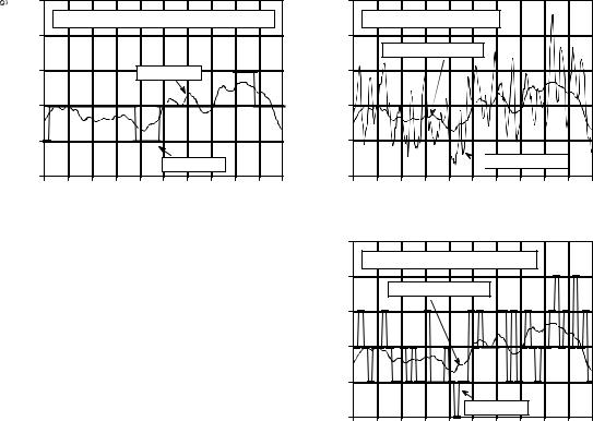
Figure 3-3 shows several sinusoids before and after digitization. The continuous line represents the analog signal entering the ADC, while the square markers are the digital signal leaving the ADC. In (a), the analog signal is a constant DC value, a cosine wave of zero frequency. Since the analog signal is a series of straight lines between each of the samples, all of the information needed to reconstruct the analog signal is contained in the digital data. According to our definition, this is proper sampling.
40 |
The Scientist and Engineer's Guide to Digital Signal Processing |
The sine wave shown in (b) has a frequency of 0.09 of the sampling rate. This might represent, for example, a 90 cycle/second sine wave being sampled at 1000 samples/second. Expressed in another way, there are 11.1 samples taken over each complete cycle of the sinusoid. This situation is more complicated than the previous case, because the analog signal cannot be reconstructed by simply drawing straight lines between the data points. Do these samples properly represent the analog signal? The answer is yes, because no other sinusoid, or combination of sinusoids, will produce this pattern of samples (within the reasonable constraints listed below). These samples correspond to only one analog signal, and therefore the analog signal can be exactly reconstructed. Again, an instance of proper sampling.
In (c), the situation is made more difficult by increasing the sine wave's frequency to 0.31 of the sampling rate. This results in only 3.2 samples per sine wave cycle. Here the samples are so sparse that they don't even appear to follow the general trend of the analog signal. Do these samples properly represent the analog waveform? Again, the answer is yes, and for exactly the same reason. The samples are a unique representation of the analog signal. All of the information needed to reconstruct the continuous waveform is contained in the digital data. How you go about doing this will be discussed later in this chapter. Obviously, it must be more sophisticated than just drawing straight lines between the data points. As strange as it seems, this is proper sampling according to our definition.
In (d), the analog frequency is pushed even higher to 0.95 of the sampling rate, with a mere 1.05 samples per sine wave cycle. Do these samples properly represent the data? No, they don't! The samples represent a different sine wave from the one contained in the analog signal. In particular, the original sine wave of 0.95 frequency misrepresents itself as a sine wave of 0.05 frequency in the digital signal. This phenomenon of sinusoids changing frequency during sampling is called aliasing. Just as a criminal might take on an assumed name or identity (an alias), the sinusoid assumes another frequency that is not its own. Since the digital data is no longer uniquely related to a particular analog signal, an unambiguous reconstruction is impossible. There is nothing in the sampled data to suggest that the original analog signal had a frequency of 0.95 rather than 0.05. The sine wave has hidden its true identity completely; the perfect crime has been committed! According to our definition, this is an example of improper sampling.
This line of reasoning leads to a milestone in DSP, the sampling theorem. Frequently this is called the Shannon sampling theorem, or the Nyquist sampling theorem, after the authors of 1940s papers on the topic. The sampling theorem indicates that a continuous signal can be properly sampled, only if it does not contain frequency components above one-half of the sampling rate. For instance, a sampling rate of 2,000 samples/second requires the analog signal to be composed of frequencies below 1000 cycles/second. If frequencies above this limit are present in the signal, they will be aliased to frequencies between 0 and 1000 cycles/second, combining with whatever information that was legitimately there.
Chapter 3- ADC and DAC |
41 |
3
a. Analog frequency = 0.0 (i.e., DC)
2 

1
Amplitude |
0 |
|
-1
-2
-3
Time (or sample number)
|
3 |
|
|
c. Analog frequency = 0.31 of sampling rate |
|
|
2 |
|
Amplitude |
1 |
|
0 |
||
|
||
|
-1 |
|
|
-2 |
|
|
-3 |
Time (or sample number)
|
3 |
|
|
b. Analog frequency = 0.09 of sampling rate |
|
|
2 |
|
Amplitude |
1 |
|
0 |
||
|
||
|
-1 |
|
|
-2 |
|
|
-3 |
|
|
Time (or sample number) |
|
|
3 |
|
|
d. Analog frequency = 0.95 of sampling rate |
|
|
2 |
|
Amplitude |
1 |
|
0 |
||
|
||
|
-1 |
|
|
-2 |
|
|
-3 |
Time (or sample number)
FIGURE 3-3
Illustration of proper and improper sampling. A continuous signal is sampled properly if the samples contain all the information needed to recreate the original waveform. Figures (a), (b), and (c) illustrate proper sampling of three sinusoidal waves. This is certainly not obvious, since the samples in (c) do not even appear to capture the shape of the waveform. Nevertheless, each of these continuous signals forms a unique one-to-one pair with its pattern of samples. This guarantees that reconstruction can take place. In (d), the frequency of the analog sine wave is greater than the Nyquist frequency (one-half of the sampling rate). This results in aliasing, where the frequency of the sampled data is different from the frequency of the continuous signal. Since aliasing has corrupted the information, the original signal cannot be reconstructed from the samples.
Two terms are widely used when discussing the sampling theorem: the Nyquist frequency and the Nyquist rate. Unfortunately, their meaning is not standardized. To understand this, consider an analog signal composed of frequencies between DC and 3 kHz. To properly digitize this signal it must be sampled at 6,000 samples/sec (6 kHz) or higher. Suppose we choose to sample at 8,000 samples/sec (8 kHz), allowing frequencies between DC and 4 kHz to be properly represented. In this situation there are four important frequencies: (1) the highest frequency in the signal, 3 kHz; (2) twice this frequency, 6 kHz; (3) the sampling rate, 8 kHz; and (4) one-half the sampling rate, 4 kHz. Which of these four is the Nyquist frequency and which is the Nyquist rate? It depends who you ask! All of the possible combinations are
42 |
The Scientist and Engineer's Guide to Digital Signal Processing |
used. Fortunately, most authors are careful to define how they are using the terms. In this book, they are both used to mean one-half the sampling rate.
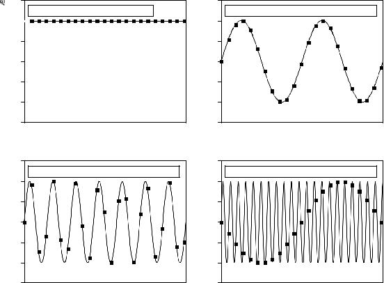
Figure 3-4 shows how frequencies are changed during aliasing. The key point to remember is that a digital signal cannot contain frequencies above one-half the sampling rate (i.e., the Nyquist frequency/rate). When the frequency of the continuous wave is below the Nyquist rate, the frequency of the sampled data is a match. However, when the continuous signal's frequency is above the Nyquist rate, aliasing changes the frequency into something that can be represented in the sampled data. As shown by the zigzagging line in Fig. 3-4, every continuous frequency above the Nyquist rate has a corresponding digital frequency between zero and one-half the sampling rate. If there happens to be a sinusoid already at this lower frequency, the aliased signal will add to it, resulting in a loss of information. Aliasing is a double curse; information can be lost about the higher and the lower frequency. Suppose you are given a digital signal containing a frequency of 0.2 of the sampling rate. If this signal were obtained by proper sampling, the original analog signal must have had a frequency of 0.2. If aliasing took place during sampling, the digital frequency of 0.2 could have come from any one of an infinite number of frequencies in the analog signal: 0.2, 0.8, 1.2, 1.8, 2.2, þ .
Just as aliasing can change the frequency during sampling, it can also change the phase. For example, look back at the aliased signal in Fig. 3-3d. The aliased digital signal is inverted from the original analog signal; one is a sine wave while the other is a negative sine wave. In other words, aliasing has changed the frequency and introduced a 180E phase shift. Only two phase shifts are possible: 0E (no phase shift) and 180E (inversion). The zero phase shift occurs for analog frequencies of 0 to 0.5, 1.0 to 1.5, 2.0 to 2.5, etc. An inverted phase occurs for analog frequencies of 0.5 to 1.0, 1.5 to 2.0, 2.5 to 3.0, and so on.
Now we will dive into a more detailed analysis of sampling and how aliasing occurs. Our overall goal is to understand what happens to the information when a signal is converted from a continuous to a discrete form. The problem is, these are very different things; one is a continuous waveform while the other is an array of numbers. This "apples-to-oranges" comparison makes the analysis very difficult. The solution is to introduce a theoretical concept called the impulse train.
Figure 3-5a shows an example analog signal. Figure (c) shows the signal sampled by using an impulse train. The impulse train is a continuous signal consisting of a series of narrow spikes (impulses) that match the original signal at the sampling instants. Each impulse is infinitesimally narrow, a concept that will be discussed in Chapter 13. Between these sampling times the value of the waveform is zero. Keep in mind that the impulse train is a theoretical concept, not a waveform that can exist in an electronic circuit. Since both the original analog signal and the impulse train are continuous waveforms, we can make an "apples-apples" comparison between the two.
Chapter 3- ADC and DAC |
43 |
|
DC |
Nyquist |
|
|
|
|
|
Frequency |
|
|
|
|
|
|
|
GOOD |
|
ALIASED |
|
|
|
|
|
|
|
|
|
frequency |
0.5 |
|
|
|
|
|
0.4 |
|
|
|
|
|
|
|
|
|
|
|
|
|
|
0.3 |
|
|
|
|
|
Digital |
0.2 |
|
|
|
|
|
0.1 |
|
|
|
|
|
|
|
|
|
|
|
|
|
|
0.0 |
|
|
|
|
|
|
0.0 |
0.5 |
1.0 |
1.5 |
2.0 |
2.5 |
Continuous frequency (as a fraction of the sampling rate)
Digital phase (degrees)
270  180
180
90
0 -90
0.0 |
0.5 |
1.0 |
1.5 |
2.0 |
2.5 |
Continuous frequency (as a fraction of the sampling rate)
FIGURE 3-4
Conversion of analog frequency into digital frequency during sampling. Continuous signals with a frequency less than one-half of the sampling rate are directly converted into the corresponding digital frequency. Above one-half of the sampling rate, aliasing takes place, resulting in the frequency being misrepresented in the digital data. Aliasing always changes a higher frequency into a lower frequency between 0 and 0.5. In addition, aliasing may also change the phase of the signal by 180 degrees.
Now we need to examine the relationship between the impulse train and the discrete signal (an array of numbers). This one is easy; in terms of information content, they are identical. If one is known, it is trivial to calculate the other. Think of these as different ends of a bridge crossing between the analog and digital worlds. This means we have achieved our overall goal once we understand the consequences of changing the waveform in Fig. 3-5a into the waveform in Fig. 3.5c.
Three continuous waveforms are shown in the left-hand column in Fig. 3-5. The corresponding frequency spectra of these signals are displayed in the righthand column. This should be a familiar concept from your knowledge of electronics; every waveform can be viewed as being composed of sinusoids of varying amplitude and frequency. Later chapters will discuss the frequency domain in detail. (You may want to revisit this discussion after becoming more familiar with frequency spectra).
Figure (a) shows an analog signal we wish to sample. As indicated by its frequency spectrum in (b), it is composed only of frequency components between 0 and about 0.33 fs, where fs is the sampling frequency we intend to
44 |
The Scientist and Engineer's Guide to Digital Signal Processing |
use. For example, this might be a speech signal that has been filtered to remove all frequencies above 3.3 kHz. Correspondingly, fs would be 10 kHz (10,000 samples/second), our intended sampling rate.
Sampling the signal in (a) by using an impulse train produces the signal shown in (c), and its frequency spectrum shown in (d). This spectrum is a duplication of the spectrum of the original signal. Each multiple of the sampling frequency, fs, 2fs, 3fs, 4fs, etc., has received a copy and a left-for- right flipped copy of the original frequency spectrum. The copy is called the upper sideband, while the flipped copy is called the lower sideband. Sampling has generated new frequencies. Is this proper sampling? The answer is yes, because the signal in (c) can be transformed back into the signal in (a) by eliminating all frequencies above ½f s. That is, an analog low-pass filter will convert the impulse train, (b), back into the original analog signal, (a).
If you are already familiar with the basics of DSP, here is a more technical explanation of why this spectral duplication occurs. (Ignore this paragraph if you are new to DSP). In the time domain, sampling is achieved by multiplying the original signal by an impulse train of unity amplitude spikes. The frequency spectrum of this unity amplitude impulse train is also a unity amplitude impulse train, with the spikes occurring at multiples of the sampling frequency, fs, 2fs, 3fs, 4fs, etc. When two time domain signals are multiplied, their frequency spectra are convolved. This results in the original spectrum being duplicated to the location of each spike in the impulse train's spectrum. Viewing the original signal as composed of both positive and negative frequencies accounts for the upper and lower sidebands, respectively. This is the same as amplitude modulation, discussed in Chapter 10.
Figure (e) shows an example of improper sampling, resulting from too low of sampling rate. The analog signal still contains frequencies up to 3.3 kHz, but the sampling rate has been lowered to 5 kHz. Notice that fS , 2fS , 3fS þ along the horizontal axis are spaced closer in (f) than in (d). The frequency spectrum, (f), shows the problem: the duplicated portions of the spectrum have invaded the band between zero and one-half of the sampling frequency. Although (f) shows these overlapping frequencies as retaining their separate identity, in actual practice they add together forming a single confused mess. Since there is no way to separate the overlapping frequencies, information is lost, and the original signal cannot be reconstructed. This overlap occurs when the analog signal contains frequencies greater than one-half the sampling rate, that is, we have proven the sampling theorem.
Digital-to-Analog Conversion
In theory, the simplest method for digital-to-analog conversion is to pull the samples from memory and convert them into an impulse train. This is