

Литература / Advanced Digital Signal Processing and Noise Reduction (Saeed V. Vaseghi) / 04 - Bayesian estimation
.pdfBayesian Classification |
129 |
image recognition), the choice of the pattern features and models affects the classification error. The design of an efficient classification for pattern recognition depends on a number of factors, which can be listed as follows:
(1)Extraction and transformation of a set of discriminative features from the signal that can aid the classification process. The features need to adequately characterise each class and emphasise the difference between various classes.
(2)Statistical modelling of the observation features for each class. For Bayesian classification, a posterior probability model for each class should be obtained.
(3)Labelling of an unlabelled signal with one of the N classes.
4.6.1 Binary Classification
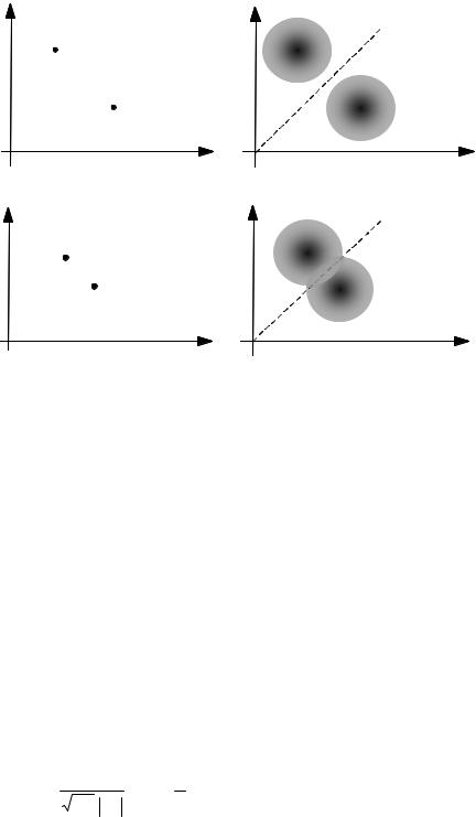
The simplest form of classification is the labelling of an observation with one of two classes of signals. Figures 4.17(a) and 4.17(b) illustrate two examples of a simple binary classification problem in a two-dimensional signal space. In each case, the observation is the result of a random mapping (e.g. signal plus noise) from the binary source to the continuous observation space. In Figure 4.17(a), the binary sources and the observation space associated with each source are well separated, and it is possible to make an error-free classification of each observation. In Figure 4.17(b) there is less distance between the mean of the sources, and the observation signals have a greater spread. This results in some overlap of the signal spaces and classification error can occur. In binary classification, a signal x is labelled with the class that scores the higher a posterior probability:
C
( ) >1 ( )
PC X C1 x < PC X C2 x
C2
Using Bayes’ rule Equation (4.125) can be rewritten as
|
|
|
|
|
|
|
|
|
C1 |
|
|
|
|
|
|
|
|
|
|
|
|
P |
(C |
)f |
X |
|
C |
(x |
|
C |
) > P |
(C |
2 |
)f |
X |
|
C |
(x |
|
C |
2 |
) |
|
|
|
|
|
||||||||||||||||||
|
|
||||||||||||||||||||
C |
1 |
|
|
|
|
1 |
< |
C |
|
|
|
|
|
|
|
||||||
|
|
|
|
|
|
|
|
|
C2 |
|
|
|
|
|
|
|
|
|
|
|
|
(4.125)
(4.126)
Letting PC(C1)=P1 and PC(C2)=P2, Equation (4.126) is often written in terms of a likelihood ratio test as
130 |
|
Bayesian Estimation |
s1 Discrete source space |
y1 |
Noisy observation space |
(a) |
s2 |
y2 |
|
s |
y1 |
|
1 |
|
(b) |
s2 |
y2 |
Figure 4.17 Illustration of binary classification: (a) the source and observation spaces are well separated, (b) the observation spaces overlap.
|
|
|
|
|
|
|
|
|
C |
|
|
|
|
|
|
|
|
||
f X |
|
C (x |
C1 ) >1 |
||||||
|
|||||||||
|
|
|
|
|
|
|
< |
||
f X |
|
C |
(x |
|
|
C2 ) |
|||
|
|
||||||||
|
|||||||||
|
|
|
|
|
|
|
|
|
C2 |
P2 |
(4.127) |
|
P1 |
||
|
Taking the likelihood ratio yields the following discriminant function:
|
|
|
|
|
|
|
|
|
|
|
|
|
|
|
|
C |
|
|
|
h(x) = ln f |
X |
|
C |
(x |
|
C |
)− ln f |
X |
|
C |
(x |
|
C |
2 |
) |
>1 |
ln |
P2 |
(4.128) |
|
|
|
|
||||||||||||||||
|
|
|
|
1 |
|
|
|
|
|
|
< |
|
P1 |
|
|||||
|
|
|
|
|
|
|
|
|
|
|
|
|
|
|
|
C2 |
|
|
|
|
|
|
|
|
|
|
|
|
|
|
|
|
|
|
|
|
|
|
Now assume that the signal in each class has a Gaussian distribution with a probability distribution function given by
|
|
C (x |
|
)= |
1 |
|
1 |
(x − µi )T Σ i−1 |
|
|
|
|
|
|
|
|
|||||||
f X |
|
ci |
|
exp − |
|
(x − µi ) |
, i=1,2 |
(4.129) |
|||
|
|
|
|||||||||
|
|
|
|
|
2π Σ i |
|
2 |
|
|
|
|
Bayesian Classification |
|
|
|
|
|
|
|
|
|
|
|
|
|
|
|
131 |
||||||
From Equations |
(4.128) |
and (4.129), |
the |
|
discriminant |
function |
h(x) |
|||||||||||||||
becomes |
|
|
|
|
|
|
|
|
|
|
|
|
|
|
|
|
|
|
|
|
|
|
|
|
|
|
|
|
|
|
|
|
|
|
|
|
|
|
|
|
|
C1 |
|
|
|
h(x) = − |
1 |
|
T |
−1 |
|
|
1 |
|
|
T |
−1 |
|
|
Σ 2 |
> |
|
P2 |
|||||
|
(x − µ1 ) |
|
Σ1 |
(x − µ1 ) + |
|
(x − µ 2 ) |
|
Σ 2 |
|
(x − µ 2 ) + ln |
|
|
|
|
|
|
ln |
|
|
|||
2 |
|
2 |
|
|
|
|
Σ1 |
|
< |
P1 |
||||||||||||
|
|
|
|
|
||||||||||||||||||
|
|
|
|
|
|
|
|
|
|
|
|
|
|
|
|
|
|
|
C2 |
|
|
|
|
|
|
|
|
|
|
|
|
|
|
|
|
|
|
|
|
(4.130) |
|||||
Example 4.10 For two Gaussian-distributed classes of scalar-valued signals with distributions given by N (x(m),µ1,σ 2 ) and N (x(m),µ2 ,σ 2 ) , and equal class probability P1=P2=0.5, the discrimination function of Equation (4.130) becomes
|
µ |
2 − |
µ1 |
|
|
µ |
|
C |
|
|
|
|
1 |
22 − µ12 >1 |
|
||||||
h(x(m)) = |
|
|
|
x(m) + |
|
|
|
|
< 0 |
(4.131) |
|
σ 2 |
|
2 |
|
|
σ 2 |
||||
|
|
|
|
|
|
C2 |
|
|||
|
|
|
|
|
|
|
|
|
|
|
Hence the rule for signal classification becomes
C |
µ1 |
+ |
µ2 |
|
<1 |
(4.132) |
|||
x(m) > |
|
2 |
|
|
C2 |
|
|
|
|
|
|
|
|
The signal is labelled with class C1 if x(m)< (µ1 + µ2 ) / 2 and as class C2 otherwise.
4.6.2 Classification Error
Classification errors are due to the overlap of the distributions of different classes of signals. This is illustrated in Figure 4.16 for the binary classification of a scalar-valued signal and in Figure 4.17 for the binary classification of a two-dimensional signal. In each figure the overlapped area gives a measure of classification error. The obvious solution for reducing the classification error is to reduce the overlap of the distributions. This may be achieved by increasing the distance between the mean values of various classes or by reducing the variance of each class. In the binary classification of a scalar-valued variable x, the probability of classification error is given by

132 |
|
|
|
|
|
|
|
|
|
|
|
|
|
|
Bayesian Estimation |
P(Error |
|
x) = P(C1 )P(x > Thrsh | x C1 ) + P(C2 )P(x > Thrsh | x C2 ) (4.133) |
|||||||||||||
|
|||||||||||||||
For two Gaussian-distributed |
classes of scalar-valued signals with pdfs |
||||||||||||||
N (x(m),µ |
,σ 2 ) and N (x(m),µ |
2 |
, |
σ 2 ) , Equation (4.133) becomes |
|||||||||||
1 |
1 |
|
|
2 |
|
|
|
|
|
|
|||||
|
|
|
|
|
∞ |
|
|
|
|
|
|
|
|
2 |
|
P(Error |
|
x) = P(C1 ) ∫ |
|
1 |
|
|
|
|
|
(x − µ1 ) |
|
||||
|
|
|
|
|
|
||||||||||
|
2π σ1 |
exp − |
2 |
|
dx |
||||||||||
|
|
||||||||||||||
|
|
|
|
|
Thrsh |
|
|
|
2σ1 |
|
|
||||
|
|
|
|
|
|
|
|
|
|
|
|
|
|
|
(4.134) |
|
|
|
|
|
Thrsh |
|
|
|
|
|
|
|
2 |
|
|
|
|
|
|
|
+ P(C2 ) ∫ |
|
1 |
|
|
− |
(x − µ2 ) |
|
|
||
|
|
|
|
|
2π σ 2 |
|
|
2 |
dx |
||||||
|
|
|
|
|
−∞ |
|
|
|
2σ 2 |
|
|
||||
where the parameter Thrsh is the classification threshold.
4.6.3 Bayesian Classification of Discrete-Valued Parameters
Let the set Θ={θi, i =1, ..., M} denote the values that a discrete P- dimensional parameter vector θ can assume. In general, the observation space Y associated with a discrete parameter space Θ may be a discretevalued or a continuous-valued space. Assuming that the observation space is continuous, the pdf of the parameter vector θi, given observation vector y , may be expressed, using Bayes’ rule, as
PΘ|Y (θi | y) = |
fY |Θ ( y|θ i )PΘ (θi ) |
|
|
(4.135) |
|
|
||
|
fY ( y) |
|
For the case when the observation space Y is discrete-valued, the probability density functions are replaced by the appropriate probability mass functions. The Bayesian risk in selecting the parameter vector θi given the observation y is defined as
M |
|
R (θi | y) = ∑C(θi |θ j )PΘ|Y (θ j | y) |
(4.136) |
j=1 |
|
where C(θi|θj) is the cost of selecting the parameter θi when the true parameter is θj. The Bayesian classification Equation (4.136) can be
Bayesian Classification |
133 |
employed to obtain the maximum a posteriori, the maximum likelihood and the minimum mean square error classifiers.
4.6.4 Maximum A Posteriori Classification
MAP classification corresponds to Bayesian classification with a uniform cost function defined as
C(θ i |θ j ) = 1− δ (θ i ,θ j ) |
(4.137) |
where δ(·) is the delta function. Substitution of this cost function in the Bayesian risk function yields
M |
|
R MAP (θ i | y) =∑ |
[1 − δ (θ i ,θ j )] PΘ | y (θ j | y) |
j=1 |
(4.138) |
= 1 − PΘ | y (θ i | y)
Note that the MAP risk in selecting θi is the classification error probability; that is the sum of the probabilities of all other candidates. From Equation (4.138) minimisation of the MAP risk function is achieved by maximisation of the posterior pmf:
θˆ |
( y) = arg max P |
(θ |
i |
| y) |
MAP |
Θ |Y |
|
|
|
|
θi |
|
|
(4.139) |
|
= arg max PΘ (θ i ) fY |Θ ( y |θ i ) |
|||
|
θi |
|
|
|
4.6.5 Maximum-Likelihood (ML) Classification
The ML classification corresponds to Bayesian classification when the parameter θ has a uniform prior pmf and the cost function is also uniform:
|
|
|
|
M |
|
|
|
|
|
1 |
|
|
(y | θ |
|
)P |
|
|
|
R |
|
(θ |
|
| y) =∑[1 − δ (θ |
|
,θ |
|
)] |
f |
|
|
(θ |
|
) |
||||
|
|
|
|
fY ( y) |
|
|
|
|||||||||||
|
ML |
|
i |
= |
|
i |
|
j |
|
|
Y |Θ |
|
j |
Θ |
|
j |
|
|
|
|
|
|
j 1 |
|
|
|
|
|
|
|
|
|
|
|
|
|
(4.140) |
|
|
|
|
|
1 |
|
|
|
|
|
|
|
|
|
|
|
|
|
|
|
|
|
= 1 − |
|
fY |θ (y | θi )PΘ |
|
|
|
|
|
|
|
|||||
|
|
|
|
|
|
|
|
|
|
|
|
|
||||||
|
|
|
|
fY ( y) |
|
|
|
|
|
|
|
|
||||||
134 Bayesian Estimation
where PΘ is the uniform pmf of θ. Minimisation of the ML risk function (4.140) is equivalent to maximisation of the likelihood f Y|Θ (y|θi )
θˆML ( y) = argmax fY|Θ ( y |θi ) |
(4.141) |
θi |
|
4.6.6 Minimum Mean Square Error Classification
The Bayesian minimum mean square error classification results from minimisation of the following risk function:
|
|
|
|
M |
|
|
|
|
|
|
|
|
|
|
|
|
||
R |
MMSE |
(θ |
i |
| y) = ∑ |
|
θ |
i |
−θ |
j |
|
2 P |
|
(θ |
j |
| y) |
(4.142) |
||
|
|
|||||||||||||||||
|
|
j=1 |
|
|
|
|
|
|
Θ|Y |
|
|
|
|
|||||
|
|
|
|
|
|
|
|
|
|
|
|
|
|
|
|
|
|
|
For the case when |
PΘ |Y (θ j| y) is not available, the MMSE classifier is |
|||||||||||||||||
given by |
|
|
|
|
|
|
|
|
|
|
|
|
|
|
|
|
|
|
|
θˆMMSE |
( y) = arg min |
|
θ i −θ ( y) |
|
2 |
|
|
(4.143) |
|||||||||
|
|
|
|
|
||||||||||||||
|
|
|
|
θ i |
|
|
|
|
|
|
|
|
|
|
|
|
||
where θ(y) is an estimate based on the observation y. |
|
|
||||||||||||||||
4.6.7 Bayesian Classification of Finite State Processes
In this section, the classification problem is formulated within the framework of a finite state random process. A finite state process is composed of a probabilistic chain of a number of different random processes. Finite state processes are used for modelling non-stationary signals such as speech, image, background acoustic noise, and impulsive noise as discussed in Chapter 5.
Consider a process with a set of M states denoted as S={s1, s2, . . ., sM}, where each state has some distinct statistical property. In its simplest form, a state is just a single vector, and the finite state process is equivalent to a discrete-valued random process with M outcomes. In this case the Bayesian state estimation is identical to the Bayesian classification of a signal into one of M discrete-valued vectors. More generally, a state generates continuous-valued, or discrete-valued vectors from a pdf, or a pmf, associated with the state. Figure 4.18 illustrates an M-state process, where the output of the ith state is expressed as

Bayesian Classification |
135 |
x(m) = hi (θ i , e(m)), i= 1, . . ., M |
(4.144) |
where in each state the signal x(m) is modelled as the output of a statedependent function hi(·) with parameter θi, input e(m) and an input pdf fEi(e(m)). The prior probability of each state is given by
|
M |
|
|
P (si ) = E[N(si )] |
E ∑ N(s j |
) |
(4.145) |
S |
j=1 |
|
|
|
|
|
|
where E[N(si)] is the expected number of observation from state si. The pdf of the output of a finite state process is a weighted combination of the pdf of each state and is given by
M
f X (x(m))=∑ PS (si ) f X |S (x | si ) (4.146)
i=1
In Figure 4.18, the noisy observation y(m) is the sum of the process output x(m) and an additive noise n(m). From Bayes’ rule, the posterior probability of the state si given the observation y(m) can be expressed as
x = h1 (θ, e) |
x = h2 (θ, e) |
. . . |
x = hM (θ, e) |
e f1 (e) |
e f2 (e) |
|
e fM (e) |
STATE switch
x
n
Noise  +
+
 y
y
Figure 4.18 Illustration of a random process generated by a finite state system.

136 |
|
|
|
|
|
|
|
Bayesian Estimation |
PS|Y (si |
|
y(m))= |
fY |S (y(m) |
|
si )PS (si ) |
(4.147) |
||
|
|
|||||||
|
|
|
|
|
|
|||
|
M |
|||||||
|
|
|
|
|||||
|
|
|
∑ fY |S (y(m) |
|
s j )PS (s j ) |
|
||
|
|
|
|
|
||||
|
|
|
j=1 |
|
|
|
||
In MAP classification, the state with the maximum posterior probability is selected as
sMAP (y(m)) = arg max PS|Y (si |
|
y(m)) |
(4.148) |
|
|||
si |
|
||
The Bayesian state classifier assigns C(si|sj) to the action of selecting the state function for the Bayesian classification is
a misclassification cost function si when the true state is sj. The risk given by
M |
|
R (si y(m)) = ∑C(si |s j )PS|Y (s j |y(m)) |
(4.149) |
j=1
4.6.8Bayesian Estimation of the Most Likely State Sequence
Consider the estimation of |
|
the most likely state sequence |
|||
s = [si0 ,si1 , ,siT −1 ] of |
a |
finite |
state process, given a sequence of T |
||
observation vectors Y = [y |
, y , , y |
|
]. A state sequence s, of length T, is |
||
|
0 |
1 |
T −1 |
|
|
itself a random integer-valued vector process with NT possible values. From the Bayes rule, the posterior pmf of a state sequence s, given an observation sequence Y, can be expressed as
PS|Y (si |
, , si |
| y0 |
, , yT −1) = |
fY|S ( y0 , , yT −1 | si , , si )PS (si , , si ) |
||||
0 |
T −1 |
0 |
T −1 |
|||||
|
|
|
|
|||||
0 |
T −1 |
|
|
fY ( y0 , , yT −1) |
|
|
||
|
|
|
|
|
|
|
(4.150) |
|
where PS(s) is the pmf of the state sequence s, and for a given observation sequence, the denominator f Y (y0 , , yT −1) is a constant. The Bayesian risk in selecting a state sequence si is expressed as

Bayesian Classification |
|
|
|
137 |
a00 |
|
|
|
|
S0 |
|
|
|
|
a10 |
|
a |
02 |
|
|
|
|
|
|
a01 |
a20 |
|
|
|
a12 |
|
|
|
|
S1 |
|
|
S2 |
|
a |
21 |
|
a22 |
|
a |
|
|
|
|
11 |
|
|
|
|
Figure 4.19 A three state Markov Process. |
|
|||
NT |
|
|
|
|
R (si y) = ∑C(si | s j )PS|Y (s j |
y) |
(4.151) |
||
j=1
For a statistically independent process, the state of the process at any time is independent of the previous states, and hence the conditional probability of a state sequence can be written as
|
|
T −1 |
|
|
|
PS|Y (si , |
, si |
y0 , , yT −1) = ∏ fY|S ( yk |
si |
)PS (si ) |
(4.152) |
0 |
T −1 |
k=0 |
k |
k |
|
|
|
|
|
|
where sik denotes state si at time instant k. A particular case of a finite state process is the Markov chain where the state transition is governed by a Markovian process such that the probability of the state i at time m depends on the state of the process at time m-1. The conditional pmf of a Markov state sequence can be expressed as
|
|
|
|
|
|
|
T −1 |
|
|
|
|
|
PS|Y (si |
, |
, si |
| |
y0 |
, , yT −1) = ∏ai i |
fS|Y (si | yk ) |
(4.153) |
|||
|
|
0 |
T −1 |
|
k −1 |
k |
k |
|
|
||
|
|
|
|
|
|
|
k=0 |
|
|
|
|
where |
ai |
i |
is the probability that the process moves from state |
si |
to |
||||||
|
k −1 k |
|
|
|
|
|
|
|
k −1 |
|
|
state |
sik |
Finite |
state |
random processes |
and |
computationally |
efficient |
||||
methods of state sequence estimation are described in detail in Chapter 5.
138 |
Bayesian Estimation |
4.7 Modelling the Space of a Random Process
In this section, we consider the training of statistical models for a database of P-dimensional vectors of a random process. The vectors in the database can be visualised as forming a number of clusters or regions in a P- dimensional space. The statistical modelling method consists of two steps:
(a)the partitioning of the database into a number of regions, or clusters, and
(b)the estimation of the parameters of a statistical model for each cluster. A simple method for modelling the space of a random signal is to use a set of prototype vectors that represent the centroids of the signal space. This method effectively quantises the space of a random process into a relatively small number of typical vectors, and is known as vector quantisation (VQ). In the following, we first consider a VQ model of a random process, and then extend this model to a pdf model, based on a mixture of Gaussian densities.
4.7.1 Vector Quantisation of a Random Process
In vector quantisation, the space of a random vector process X is partitioned into K clusters or regions [X1, X2, ...,XK], and each cluster Xi is represented by a cluster centroid ci. The set of centroid vectors [c1, c2, ...,cK] form a VQ code book model of the process X. The VQ code book can then be used to classify an unlabelled vector x with the nearest centroid. The codebook is searched to find the centroid vector with the minimum distance from x, then x is labelled with the index of the minimum distance centroid as
Label(x)= arg min d (x, ci ) |
(4.154) |
i |
|
where d(x, ci) is a measure of distance between the vectors x and ci. The most commonly used distance measure is the mean squared distance.
4.7.2 Design of a Vector Quantiser: K-Means Clustering
The K-means algorithm, illustrated in Figure 4.20, is an iterative method for the design of a VQ codebook. Each iteration consists of two basic steps : (a) Partition the training signal space into K regions or clusters and (b) compute the centroid of each region. The steps in K-Means method are as follows: