

RM7
.pdfSCHMIDT MODES AND ENTANGLEMENT |
17 |
|
0.9 |
|
|
0.8 |
|
coherence |
0.7 |
|
0.6 |
||
|
||
|
0.5 |
|
of |
0.4 |
|
0.3 |
||
Degree |
||
0.2 |
||
|
||
|
0.1 |
|
|
0 |
|
|
10–1 |
100 |
101 |
102 |
Crystal length, mm |
|
|
Fig. 4. Degree of coherence vs. crystal length for the pump bandwidth parameter σ = 10 ps–1.
|Ψ = ------ |
[ψ(ωo, ωe )|HV + ψ(ωe, ωo )|VH]. |
(35) |
|
1 |
s i |
s i |
|
2 |
|
|
|
The first right-hand term is the probability amplitude that the ordinary and the extraordinary ray will be the signal and the idler mode, respectively. The second term is the probability amplitude that the ordinary and
extraordinary rays will be the idler and signal modes, respectively.
Assume that
|
|
|
|
|
|
|
|
|
|
0 |
|
|
|
|
|
|
0 |
|
|
|
|
|
|
|
|
|
|
|
|
|
|
|
|
|
|
|
|
|
|
|V |
|e |
= |HV = |
|
1 |
, |
|e |
|
= |
|VH = |
|
0 . |
||||||||
|H = |
1 , |
= 0 |
, |
||||||||||||||||
0 |
|
1 |
|
1 |
|
|
|
|
|
2 |
|
|
|
|
1 |
|
|||
|
|
|
|
|
|
0 |
|
|
|
|
|
|
|
||||||
|
|
|
|
|
|
|
|
|
|
0 |
|
|
|
|
|
|
0 |
||
Then Eq. (35) becomes |
|
|
|
|
|
|
|
|
|
|
|
|
|
|
|
|
|
|
|
|
|
|
|
|
|
|
|
|
|
|
|
|
|
|
|
|
|
||
|
|
|
|Ψ |
= |
1 |
[ψpq|e1 + |
ψqp|e2]. |
|
|
|
|
|
|
|
(36) |
||||
|
|
|
|
|
|
|
|
|
|
||||||||||
|
|
|
------ |
|
|
|
|
|
|
|
|||||||||
|
|
|
|
|
2 |
|
|
|
|
|
|
|
|
|
|
|
|
|
|
The frequency parts of ψpq and ψqp are adjoint |
|
|
|||||||||||||||||
The bra vector corresponding to ket vector (36) |
|||||||||||||||||||
matrices produced by discretization of Eq. (34). |
|
is |
|
|
|
|
|
|
|
|
|
|
|
||||||
|
|
|
Ψ| |
= |
1 |
[ψ*pq e1| + |
ψqp* e2|]. |
|
|
|
|
|
|
|
(37) |
||||
|
|
|
|
|
|
|
|
|
|
||||||||||
|
|
|
------ |
|
|
|
|
|
|
|
|||||||||
|
|
|
|
|
2 |
|
|
|
|
|
|
|
|
|
|
|
|
|
|
If we are interested in photon polarization rather than frequency, we construct a polarization density matrix from an overall density matrix by
summation over the frequency degrees of freedom according to standard rules of quantum mechanics [14]:
ρˆ = Trpq(|ΨΨ|). |
(38) |
|
|
RUSSIAN MICROELECTRONICS Vol. 35 No. 1 2006
18 |
|
|
|
|
|
BOGDANOV et al. |
|
|
|
|
|
|
|
|
||
|
0.12 |
L = 0.5 mm, σ = 10 ps–1, Mode 1, lam = 0.339 |
0.10 |
|
Mode 3, lam = 0.153 |
|
|
|||||||||
|
|
|
|
(a) |
Ordinary |
|
0.08 |
|
|
|
(c) |
|
|
|
|
|
|
0.10 |
|
|
|
|
|
|
|
|
|
|
|
|
|||
|
|
|
|
|
0.06 |
|
|
|
|
|
|
|
|
|||
|
|
|
|
Extraordinary |
|
|
|
|
|
|
|
|
|
|||
|
|
|
|
|
|
|
|
|
|
|
|
|
|
|||
|
0.08 |
|
|
|
|
|
|
0.04 |
|
|
|
|
|
|
|
|
Ψ |
0.06 |
|
|
|
|
|
|
0.02 |
|
|
|
|
|
|
|
|
|
|
|
|
|
|
0 |
|
|
|
|
|
|
|
|
||
|
|
|
|
|
|
|
|
|
|
|
|
|
|
|
||
|
|
|
|
|
|
|
|
|
|
|
|
|
|
|
|
|
|
0.04 |
|
|
|
|
|
|
–0.02 |
|
|
|
|
|
|
|
|
|
0.02 |
|
|
|
|
|
|
–0.04 |
|
|
|
|
|
Ordinary |
|
|
|
|
|
|
|
|
|
–0.06 |
|
|
|
|
|
Extraordinary |
|
||
|
|
|
|
|
|
|
|
|
|
|
|
|
|
|
|
|
|
0 |
|
–2 |
0 |
2 |
4 |
6 p(q) |
–0.08 |
–6 |
– 4 |
–2 |
0 |
2 |
4 |
6 |
8 |
|
–8 – 6 – 4 |
–8 |
||||||||||||||
|
0.10 |
Mode 2, lam = 0.229 |
|
|
|
0.10 |
|
Mode 4, lam = 0.101 |
|
|
|
|||||
|
|
(b) |
|
Ordinary |
|
|
|
(d) |
|
|
|
|
|
|||
|
0.08 |
|
|
|
0.08 |
|
|
|
|
Ordinary |
|
|||||
|
|
|
|
|
|
|
|
|
|
|
||||||
|
|
|
|
Extraordinary |
|
|
|
|
|
|
|
|||||
|
0.06 |
|
|
|
|
0.06 |
|
|
|
|
|
Extraordinary |
|
|||
|
|
|
|
|
|
|
|
|
|
|
|
|
||||
|
0.04 |
|
|
|
|
|
|
0.04 |
|
|
|
|
|
|
|
|
|
0.02 |
|
|
|
|
|
|
0.02 |
|
|
|
|
|
|
|
|
|
0 |
|
|
|
|
|
|
0 |
|
|
|
|
|
|
|
|
–0.02 |
|
|
|
|
|
|
-0.02 |
|
|
|
|
|
|
|
|
|
–0.04 |
|
|
|
|
|
|
–0.04 |
|
|
|
|
|
|
|
|
|
–0.06 |
|
|
|
|
|
|
–0.06 |
|
|
|
|
|
|
|
|
|
–0.08 |
|
|
|
|
|
|
–0.08 |
|
|
|
|
|
|
|
|
|
–0.10–8 |
– 6 – 4 –2 |
0 |
2 4 |
6 |
8 |
|
–0.10–8 |
–6 |
– 4 –2 |
0 |
2 |
4 |
6 |
8 |
|
|
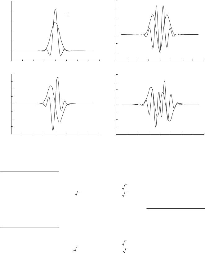
Fig. 5. Comparison of modes of an ordinary and an extraordinary ray for a high degree of coherence, F = 0.97 (small crystal length and/or small pump bandwidth). The panels refer to modes (a) 1, (b) 2, (c) 3, and (d) 4.
We thus obtain |
|
|
|
|
|
|
|
|
|
|
|
0 |
0 |
0 0 |
|
|
|
|
1 |
|
0 |
1 |
F 0 |
|
|
|
ρˆ = |
|
|
. |
(39) |
||||
-- |
|
|
|
|
|
|||
|
2 |
0 |
F* 1 0 |
|
|
|||
|
|
|
|
|
|
|||
|
|
|
0 |
0 |
0 0 |
|
|
|
Here, F represents the degree of coherence (between the two modes) for the biphotonic state. It is given by
F = ∑ψpqψqp* = Tr(ψψ*), |
(40) |
pq |
|
the asterisk denoting complex rather than Hermitian conjugation. Note that the normalization condition implies Tr(ψψ+) = 1.
In our case, F is a real number such that 0 ≤ F ≤ 1. If F = 1, we have a pure state:
|
|
|
0 |
|
|
|
|
|
|
|
|
1 |
[|HV + |VH] = |
|
1/ |
2 |
|
------ |
|
. |
|||
2 |
|
|
1/ |
2 |
|
|
|
|
0 |
|
|
|
|
|
|
|
RUSSIAN MICROELECTRONICS Vol. 35 No. 1 2006
Ψ
0.20
0.15
0.10
0.05
0
–0.05
–8
0.20
0.15
0.10
0.05
0
–0.05
–0.10
–0.15
–0.20
–8
|
SCHMIDT MODES AND ENTANGLEMENT |
19 |
||
L = 4 mm, σ = 10 ps–1, Mode 1, lam = 0.635 |
0.20 |
Mode 3, lam = 0.075 |
|
|
(a) |
Ordinary |
0.15 |
(c) |
|
|
|
|||
|
Extraordinary |
0.10 |
|
|
|
|
|
|
|
|
|
0.05 |
|
|
|
|
0 |
|
|
|
|
|
|
|
|
|
|
– 0.05 |
|
|
|
|
|
|
|
|
|
|
|
|
|
|
|
|
– 0.10 |
|
|
|
|
|
|
|
|
– 6 |
– 4 |
– 2 |
0 |
2 |
4 |
6 p(q) |
– 0.15 |
– 6 |
– 4 |
– 2 |
0 |
2 |
4 |
6 |
8 |
|
– 8 |
||||||||||||||||
|
|
Mode 2, lam = 0.214 |
|
|
|
0.20 |
|
|
Mode 4, lam = 0.03 |
|
|
|
||||
|
(b) |
|
|
|
|
|
|
0.15 |
|
(d) |
|
|
|
|
|
|
|
|
|
|
|
|
|
|
|
|
|
|
|
|
|
||
|
|
|
|
|
|
|
|
0.10 |
|
|
|
|
|
|
|
|
|
|
|
|
|
|
|
|
0.05 |
|
|
|
|
|
|
|
|
|
|
|
|
|
|
|
|
0 |
|
|
|
|
|
|
|
|
|
|
|
|
|
|
|
|
– 0.05 |
|
|
|
|
|
|
|
|
|
|
|
|
|
|
|
|
– 0.10 |
|
|
|
|
|
|
|
|
|
|
|
|
|
|
|
|
– 0.15 |
|
|
|
|
|
|
|
|
– 6 |
– 4 |
– 2 |
0 |
2 |
4 |
6 |
8 |
– 0.20 |
– 6 |
– 4 |
– 2 |
0 |
2 |
4 |
6 |
8 |
– 8 |
||||||||||||||||
Fig. 6. Comparison of modes of an ordinary and an extraordinary ray for a low degree of coherence, F = 0.37. The panels refer to modes (a) 1, (b) 2, (c) 3, and (d) 4.
If F = 0, we have a fully incoherent mixture of the states |HV and |VH with equal weights. If 0 < F < 1,
we deal with a partially coherent polarization state formed by the state
|
|
|
0 |
|
|
|
|
|
|
|
|
1 |
[|HV + |VH] = |
|
1/ |
2 |
|
------ |
|
|
|||
2 |
|
|
1/ |
2 |
|
|
|
|
0 |
|
|
|
|
|
|
|
1 + F
with weight ------------ and the state 2
|
|
|
0 |
|
|
|
|
|
|
|
|
1 |
[|HV – |VH] |
|
1/ |
2 |
|
------ |
= |
|
|||
2 |
|
|
–1/ |
2 |
|
|
|
|
0 |
|
|
|
|
|
|
|
1 – F with weight ------------ .
2
RUSSIAN MICROELECTRONICS Vol. 35 No. 1 2006
20 |
BOGDANOV et al. |
The above discussion of mixed states could be reinforced experimentally by techniques of quantum tomography for biphotonic fields [15, 16].
Figure 4 depicts the degree of coherence F against the crystal length L for σ = 10 ps–1. Since F is actually a function of Lσ (see Eq. (33)), it is easy to calculate the F–L relationship for another value of σ.
Figure 5 compares modes of an ordinary and an extraordinary ray for a high F (small L and/or small σ). We see that the modes of the same order are close to each other if they are odd modes; otherwise, they differ in sign. The graphs are calculated for L = 0.5 mm, σ = 10 ps–1, F = 0.97, K = 5.6, and S = 3.16.
Figure 6 makes the same comparison for a lower F. The graphs are calculated for L = 4 mm, σ = 10 ps–1, F
=0.37, K = 2.2, and S = 1.8.
7.CONCLUSIONS
(i)An SVD algorithm of Schmidt-mode extraction is proposed for continuous-variable systems. It is shown to be manageable, accurate, and reliable. A comparison is made with methods used by other workers.
(ii)For an atom–photon system with spontaneous emission, the evolution of entangled states is found to be governed by a parameter approximately equal to the fine-structure constant times the atom-to-electron mass ratio.
(iii)An analysis is made of the dynamics of entanglement in the system, covering the evolution of the entanglement entropy between the atomic and photonic degrees of freedom. It is shown that in the course of emission the entanglement entropy first rises on a timescale of order the excited-state lifetime and then falls, approaching asymptotically a residual level due to the initial energy spread of the atomic packet (momentum spread squared). Analytical expressions are derived for the photonic modes.
(iv)For type-II SPDC the loss of intermodal coherence is addressed. A polarization density matrix is calculated, and a coherence parameter is introduced to allow for the difference in behavior between ordinaryand extraordinary-ray photons in a nonlinear crystal. The degree of intermodal coherence is investigated as a function of crystal length and pump bandwidth. Example Schmidt modes for different degrees of coherence are analyzed. The results obtained should be of immediate relevance to quantum-cryptography experiments.
ACKNOWLEDGMENTS
We gratefully acknowledge useful discussions of the results with B.A. Grishanin, S.P. Kulik, and all the participants in workshops on quantum information sci-
ence at the Academy’s Institute of Physics and Technology.
REFERENCES
1.Valiev, K.A. and Kokin, A.A., Kvantovye komp’yutery: nadezhdy i real’nost’ (Quantum Computers: Hopes and Reality), Moscow: RKhD, 2004, 2nd ed.
2.Chan, K.W., Law, C.K., and Eberly, J.H., Localized Sin- gle-Photon Wave Function in Free Space, Phys. Rev. Lett., 2002, vol. 88, p. 100402.
3.Law, C.K., Walmsley, I.A., and Eberly, J.H., Continuous Frequency Entanglement: Effective Finite Hilbert Space and Entropy Control, Phys. Rev. Lett., 2000, vol. 84, p. 5304.
4.Lamata, L. and Leon, J., Dealing with Entanglement of Continuous Variables: Schmidt Decomposition with Discrete Sets of Orthogonal Functions, LANL e-print archive quant-ph/0410167, 2004.
5.Fedorov, M.V., Efremov, M.A., Kazakov, A.E., et al., Spontaneous Emission of a Photon: Wave Packet Structures and Atom-Photon Entanglement, LANL e-print archive quant-ph/0412107, 2004.
6.Berestetski, V.B., Lifshitz, E.M., and Pitaevskii, L.P.,
Kvantovaya elektrodinamika (Quantum Electrodynamics), Moscow: Nauka, 1989.
7.Balashov, V.V. and Dolinov, V.K., Kurs kvantovoi mekhaniki (A Course in Quantum Mechanics), Moscow: Mosk. Gos. Univ., 1982.
8.Chan, K.W., Law, C.K., and Eberly, J.H., Quantum Entanglement in Photon-Atom Scattering, Phys. Rev. A, 2003, vol. 68, p. 022110.
9.Scully, M.O. and Zubairy, M.S., Quantum Optics, Cambridge: Cambridge Univ. Press, 1997. Translated under the title Kvantovaya optika, Moscow: Fizmatlit, 2003.
10.Klyshko, D.N., Fotony i nelineinaya optika (Photons and Nonlinear Optics), Moscow: Nauka, 1980.
11.Grice, W.P. and Walmsley, I.A., Spectral Information and Distinguishability in Type-II Down-conversion with a Broadband Pump, Phys. Rev. A, 1997, vol. 56, p. 1627.
12.Kim, Y.H., Chekhova, M.V., Kulik, S.P., et al., FirstOrder Interference of Nonclassical Light Emitted Spontaneously at Different Times, Phys. Rev. A, 2000, vol. 61, p. 051803.
13.Keller, T.E. and Rubin, M.H., Theory of Two-Photon Entanglement for Spontaneous Parametric Down-con- version Driven by a Narrow Pump Pulse, Phys. Rev. A, 1997, vol. 56, p. 1534.
14.Landau, L.D. and Lifshitz, E.M., Kvantovaya mekhanika. Nerelyativistskaya teoriya (Quantum Mechanics: Nonrelativistic Theory), Moscow: Nauka, 1974.
15.Bogdanov, Yu.I., Chekhova, M.V., Kulik, S.P., et al., Statistical Reconstruction of Qutrits, Phys. Rev. A, 2004, vol. 70, p. 042303.
16.Bogdanov, Yu.I., Chekhova, M.V., Kulik, S.P., et al., Qutrit State Engineering with Biphotons, Phys. Rev. Lett., 2004, vol. 93, p. 230503.
RUSSIAN MICROELECTRONICS Vol. 35 No. 1 2006