

PRA42303
.PDFPHYSICAL REVIEW A 70, 042303 (2004)
Statistical reconstruction of qutrits
Yu. I. Bogdanov
Russian Control System Agency, 9Angstrem,9 Moscow 124460, Russia
M. V. Chekhova, L. A. Krivitsky, S. P. Kulik, A. N. Penin, and A. A. Zhukov*
Department of Physics, Moscow M.V. Lomonosov State University, 119992 Moscow, Russia
L. C. Kwek²
National Institute of Education Nanyang Technological University, 637616 Singapore
C. H. Oh and M. K. Tey³
Department of Physics, Faculty of Science, National University of Singapore, 117542 Singapore
(Received 16 April 2004; published 5 October 2004)
We discuss a procedure of measurement followed by the reproduction of the quantum state of a three-level optical systemÐa frequencyÐand spatially degenerate two-photon ®eld. The method of statistical estimation of the quantum state based on solving the likelihood equation and analyzing the statistical properties of the obtained estimates is developed. Using the root approach of estimating quantum states, the initial two-photon state vector is reproduced from the measured fourth moments in the ®eld. The developed approach applied to quantum-state reconstruction is based on the amplitudes of mutually complementary processes. The classical algorithm of statistical estimation based on the Fisher information matrix is generalized to the case of quantum systems obeying Bohr's complementarity principle. It has been experimentally proved that biphoton-qutrit states can be reconstructed with the ®delity of 0.995±0.999 and higher.
DOI: 10.1103/PhysRevA.70.042303 |
PACS number(s): 03.67.2a, 42.50.Dv |
I. INTRODUCTION
The ability of measuring quantum states is of fundamental interest because it provides a powerful tool for the analysis of basic concepts of quantum theory, such as the fundamentally statistical nature of its predictions, the superposition principle, Bohr's complementarity principle, etc. To measure the quantum state one needs to perform some projective measurements on the state and then to apply some computation procedure to the data. The ®rst step is a genuine measurement consisting of a set of operations on the representatives of a quantum statistical (pure or mixed) ensemble. As a result of such an operation an experimentalist acquires a set of frequencies at which particular events occur. In the second step a mathematical procedure is applied to the statistical data obtained in the previous step to reconstruct the quantum state. Obviously, the complexity of the whole reconstruction procedure depends directly on the minimal number of measurements required for the reconstruction, which, in its turn, is given by the dimensionality of the state Hilbert space.
The necessity of an adequate measurement of the states of such systems is caused not only by fundamental interest but also by some applications. For example, it has been shown that the security of the key distribution in quantum cryptography is associated with the dimensionality of the Hilbert space for the states in use [1]. From this point of view certain
*Electronic address: postmast@qopt.phys.msu.su ²Electronic address: lckwek@nie.edu.sg
³Electronic address: phyohch@nus.edu.sg, phyteymk@nus.edu.sg
hopes are pinned on the three-level systems or qutrits [2±4] rather than qubits.
The present paper is devoted to state reconstruction for the optical three-level systems. The object under study is the polarization state of a frequency and spatially degenerate biphoton ®eld [5,6].
We should mention that there are other implementations of three-level optical systems. The most familiar ones deal with three-arm interferometers [7] and lower-order transverse spatial modes of optical ®eld, realized with holograms [8±10]. Polarization-entangled four-photon ®elds, which are equivalent to two entangled spin-1 particles, were studied in [11].
All these implementations belong to the art of the modern experimental technique and demonstrate the development of those quantum information branches relating to the practice. However, note that successful manipulation with quantum states implies the ability to control three important stages: state preparation, its transformation, and measurement. From this point of view, biphoton qutrits look quite promising since the mentioned stages are under the full control. The unitary transformations of biphoton polarization states as well as quantum ternary logic have been considered in [12]. Preparation of arbitrary qutrits was realized recently [13], so in the present paper we focus on the complete reconstruction of the biphoton qutrits. Although realistic tomographic procedures for measuring such quantum states were suggested earlier [14±16], this work includes the most advanced approach. Such an approach consists of statistical estimation of the experimental data based on solving the likelihood equation, the so-called root estimation technique [17]. The advantages of the root estimation method are based on the ability
1050-2947/2004/70(4)/042303(16)/$22.50 |
70 042303-1 |
©2004 The American Physical Society |
BOGDANOV et al.
to reconstruct the states in the Hilbert space of high dimensionality. The method is asymptotically effective, so it allows one to reconstruct the states with an accuracy that is most close to the accuracy achievable in principle. That is why the formalism applied to the unknown quantum states allowed us to formulate and experimentally check the fundamental statistical limits of the accuracy of state reconstruction. Practically, this is the ®rst application of the root estimation to a large set of experimental data obtained in different regimes of biphoton-state generation, which are widely used in quantum optics and quantum informationÐnamely, speaking about temporal regimes, the data under analysis related to continuous and short-pulsed biphoton sources. As to the polarization regimes, we investigated both types of phase matching (type I and type II) for producing biphotons. Among the works that closely relate to the subject of the present paper and are devoted to state reconstruction, we would like to refer to the family of papers in [18±21], where quantum tomography of qubit pairs was developed. In these works, a detailed analysis of the biphoton polarization states involved in a wide range of processes like decohering, unitary, etc., was implemented. The approach developed in these works exploits the noncollinear (and degenerate) regime for the correlated photon source. Transition to the collinear (and degenerate) regime when biphotons propagate in the single beam rather than in two beams becomes crucial. We put great emphasis on that fact because it makes possible to pass from qubits to qutrits or to a new class of states with higher dimensionality (see Sec. II).
The paper is organized as follows. In Sec. II we discuss the main properties of qutrits based on the polarization state of the biphoton ®eld. We focus on their preparation, visual representation on a Poincaré sphere, and unitary transformation by phase plates. Then we consider the coherence matrix, which characterizes completely the properties of biphoton qutrits in the fourth ®eld moments. Section III is devoted to the methods of biphoton-qutrit measurement; in particular, we introduce two quantum tomography protocols and discuss in detail their experimental implementation. We conclude this part with an analysis of statistical reconstruction for qutrits from the outcomes of mutually complementary measurements. Section IV deals with the methods of quantumstate reconstruction. Namely, we consider the least-squares and maximum-likelihood methods and apply these tools to analysis of the data obtained in quantum tomography. In the Appendix we explore the problem of statistical ¯uctuations of the state vector which is important for estimation and control of the precision and stability of quantum information.
II. QUTRITS BASED ON BIPHOTONS
A. Preparation
Biphoton ®eld is a coherent mixture of two-photon Fock states and the vacuum state [22]:
C = uvacl + |
1 |
o FkWs,kWiu1kWs,1kWil, |
s1d |
|
|||
|
2 W W |
|
|
|
|
kski |
|
where u1kWs , 1kWil denotes the state with one (signal) photon in
W ( ) W
the mode ks and one idler photon in the mode ki. The co-
PHYSICAL REVIEW A 70, 042303 (2004)
ef®cient FkWs,kWi is called the biphoton amplitude [23], because
its squared modulus gives a probability to register two pho-
W W tons in modes ks and ki.
Let us consider the collinear and frequency-degenerate
W < W v < v v v v v regime, for which ks ki, s i and s + i = p, where p
is the laser pump frequency. We further restrict our discussion to biphotons that are indistinguishable in terms of spatial, spectral, or temporal parameters. From the point of view of polarization there are three natural states of biphotons:
namely, C1 = u2 , 0l, C2 = u1 , 1l, and C3 = u0 , 2l. Here the notation u2 , 0l ; u2H , 0Vl, for example, indicates that there are
two photons in the horizontal sHd polarization mode, while no photons are present in the orthogonal vertical sVd mode. These basic states can be generated using type-I (for C1 and C3) and type-II (for C2) phase matching. Since only twophoton Fock states are considered, for the state um , nl the condition m + n = 2 must be satis®ed.
Any arbitrary pure polarization state of biphoton ®eld can be expressed in terms of three complex amplitudes c1 , c2,
and c3: |
|
ucl = c1u2,0l + c2u1,1l + c3u0,2l, |
s2d |
where cj = ucjuexphiwjj and o3j=1ucju2 = 1. The vector |
ucl |
= sc1 , c2 , c3d represents a three-state state or qutrit. |
|
There is an important note concerning the state vector (2). In principle, one can write the complete polarization state in
the form |
|
|
|
|
|
|
|
|
|
|
|
|
|
|
|
|
|
|
|
|
|
|
ucl = c |
1 |
u2 |
H |
,0 |
V |
l + c |
2 |
u1 |
V |
,1 |
H |
l + c8u1 |
H |
,1 |
V |
l + c |
3 |
u0 |
H |
,2 |
V |
l, s3d |
|
|
|
|
|
|
2 |
|
|
|
|
|
where the terms u1H , 1Vl and u1V , 1Hl might be distinguishable somehow, for example, if the photon with vertical polarization comes ®rst with respect to the photon with horizontal polarization. However, we consider a particular twomode polarization state, so photons differ in polarization only and there are no other parameters responsible for their distinguishability.
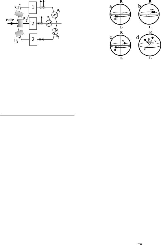
In general, to generate an arbitrary qutrit state one needs to put three nonlinear crystals separated in space into a common pump and superpose the biphoton ®elds generated by the three crystals coherently or incoherently (Fig. 1).
B. Representation of qutrits using the Poincaré sphere
Sometimes it is very convenient to use a visual representation of the state. For example, a single-photon pure polarization state (qubit) may be mapped onto the Poincaré sphere [three-dimensional (3D) Euclidian sphere]. A (pure) qubit state is determined by polar and azimuthal angles sq , fd in spherical coordinates. Any unitary polarization transformation of the qubit is represented by the corresponding rotation of the sphere. Thus, in order to learn the ®nal transformed state one just has to apply the rotation operation using certain rules.
It would be helpful to use the same visual representation of a qutrit using the Poincaré sphere. Although generalization of the Poincaré sphere for qutrits has been discussed earlier [24] we suggest an alternative approach, which allows us to manipulate with qutrits in natural 3D space rather than in
042303-2
STATISTICAL RECONSTRUCTION OF QUTRITS
FIG. 1. Preparation of an arbitrary qutrit based on biphotons, in principle. Three nonlinear crystals placed in the common pump generate biphotons with type-I (1, 3) and type-II (2) phase matching. Three attenuators suc1u2 , uc1u2 , uc3u2d and three phase shifters sw1 , w2 , w3d allow one to control three complex amplitudes c1, c2, and c3.
sophisticated 8D space. Let us map the pure polarization state of a biphoton into a pair of points on the sphere (but this is not the two-qubit case since the states uH , Vl and uV , Hl are indistinguishable). In this representation each photon forming the biphoton is plotted as a single point on the Poincaré sphere, so the qutrit-state vector is represented by
fa²sq,fda²sq8,f8d + a²sq,fda²sq8,f8dguvacl
ucl = s i i s ,
uufa²s sq,fda²i sq8,f8d + a²i sq,fda²s sq8,f8dguvacluu
s4d
where a²sqi , fid and a²sqs , fsd are the creation operators in
idler and signal |
polarization modes and |
a²sqm , fmd |
= cossqm / 2da² + eifmsinsqm / 2db² , m = i , s. Note |
that opera- |
|
tors a² ; aH² , b² ; aV² |
are creation operators |
for H- and |
V-polarized photons. |
|
|
It is well known that the number of real parameters characterizing a quantum state is determined by the dimension of
the Hilbert space ssd. For a pure state, |
|
Npure = 2s − 2, |
s5ad |
and for mixed states, |
|
Nmixed = s2 − 1. |
s5bd |
According to Eqs. (5a) and (5b), four real parameters determine completely the pure state of a qutrit, so in the Poincaré sphere representation these parameters are simply the four spherical angles sqi , fi ; qs , fsd. The links between the angles sqi , fi ; qs , fsd and the amplitudes cj = ucjuexp iwj
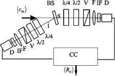
are derived in [6]. As an example three basic states C1 |
||||
= u2 , 0l, C2 = u1 , 1l, and C3 = u0 , 2l are shown in Fig. 2. It can |
||||
be shown that the polarization |
degree of |
a qutrit P |
||
= Î |
|
[6] |
|
|
uc1u2 − uc3u2 + 2uc1*c2 + c2*c3u2 |
has a clear |
geometrical |
||
meaning: it is de®ned by the angle b between the pair of points on the Poincaré sphere as seen from its center:
|
2 cossb/2d |
s6d |
P = |
1 + cos2sb/2d . |
For the states C1 and C3 the polarization degree takes values P1,3 = 1, since two points coincide on the sphere and b = 0.
PHYSICAL REVIEW A 70, 042303 (2004)
FIG. 2. Representation of a qutrit using the Poincaré sphere. (a), (b), and (c) show three basic states forming superposition (2). (d) represents the state of an arbitrary qutrit.
For the second state, C2, two points are positioned at the opposite sides of the sphere; that is why b / 2 = p / 2 and P2 = 0.
C. Transformation
Experimentally a unitary transformation of the polarization state (2) can be achieved by placing any retardation plates, rotators, etc., into the biphoton beam. The action of such elements on the state (2) is described by the matrix [12]
|
1 |
t2 |
|
|
Î |
|
|
tr |
|
|
r2 |
|
2 |
|
|
||||
|
|
|
2 |
|
|
|
|
|
|||||||||||
G = |
Î |
|
|
* |
t |
2 − |
|
r |
2 |
Î |
|
* |
r |
, |
s7d |
||||
|
|
|
|
||||||||||||||||
− 2tr |
|
u u |
|
|
|
|
u u |
|
|
2t |
|||||||||
|
r*2 |
|
− Î |
|
t*r* |
t*2 |
|
|
|
||||||||||
|
|
2 |
|
|
|
||||||||||||||
where
t = cos d + i sin d cos 2a, r = i sin d sin 2a, |
s8d |
d = psno − nedh / l is the optical thickness of the plate, h is its geometrical thickness, and a is the orientation angle between the optical axis of the plate and one of the basisÐfor example, the vertical direction.
Let us consider the action of the l / 2 plate on a particular state C' = s1 / Î2dsu2 , 0l − u0 , 2ld, when the plate is oriented at
22.5°. For the state C' there are two nonzero amplitudes c1 = c3 = 1 / Î2 and there is only one relative phase w13 ; w1 − w3 = p. Taking into account that for a l / 2 plate d = p / 2, the corresponding transmission and re¯ection coef®cients are
i |
s9d |
t = r = Î2 . |
Thus the matrix G has the form
042303-3

BOGDANOV et al. |
|
|
|
|
|
|
|
|
|
|
|
|
|
|
|
|
|
|
|
|
|
|
1 |
|
1 |
|
1 |
|
|
1 |
2 |
|
|
||||||||||
|
− |
|
|
|
|
− |
|
|
|
|
− |
|
|
|
|
|
|
||||
|
2 |
|
Î |
|
|
2 |
|
|
|||||||||||||
|
|
2 |
|
|
|||||||||||||||||
G = |
− |
1 |
|
0 |
|
|
|
|
1 |
|
. |
s10d |
|||||||||
|
|
|
|
|
|
|
|
|
|
|
|
||||||||||
|
|
|
|
|
|
|
|
|
|
|
|
||||||||||
Î2 |
|
|
Î2 |
|
|||||||||||||||||
|
|
|
|
|
|
|
|
|
|
|
|||||||||||
|
− |
|
1 |
|
|
1 |
|
|
− |
1 |
|
|
|||||||||
|
|
|
|
|
Î |
|
|
|
|
|
|
||||||||||
|
|
2 |
|
2 |
|
|
|||||||||||||||
|
|
|
2 |
|
|
|
|||||||||||||||
Hence, acting by matrix G on the state C' we get
' |
Î2 |
1− 1 |
2 1 0 |
2 |
2 |
|
|
G |
1 |
0 |
|
|
|
GC = |
|
|
0 |
= − 1 |
|
= C . |
|
|
|
||||
Note that such kind of transformations cannot change the polarization degree of a qutrit. For the state C' chosen above, as well as for the state C2, the polarization degree P is zero.
In the experiment described below we used a simpler way to generate qutrits. Biphotons were produced via collinear frequency-degenerate spontaneous parametric downconversion in a nonlinear crystal (BBO, type-I or type-II phase matching). For type-I phase matching the polarization of both created photons was vertical; i.e., the state C3 was generated. Then, this state was transformed using a quartz plate with a ®xed optical thickness. By changing the angle of the plate, the state C3 = u0H , 2Vl is transformed according to the formula ucinl = GC3. For the case of type-II phase matching the ®nal state is ucinl = GC2. Of course, the state ucinl does not involve all possible qutrit states because the transformation given by matrix (7) preserves the polarization degree. Anyway, using such a transformation, we select some subset of qutrits to work with.
Such a simple method of state preparation and transformation was chosen in order to be able to compare the results of reconstruction with the parameters of the input states, which should be known with a high accuracy. The purpose of this work is the reconstruction of the initial state ucinl.
We would like to emphasize that only pure qutrit states are accessible by this method. To create a mixed state, some more complicated method is to be used. This method allows one to create arbitrary qutrit states and it implies a possibility to introduce controlled delay between three fundamental states forming the qutrit which could exceed the coherence length of the laser pump [13].
D. Coherence matrix
We introduced only qualitative description of the qutrits based on biphotons so far. The quantitative measure characterizing the polarization properties of any single-mode state in the fourth moment in the ®eld (including the biphoton state) was proposed by Klyshko [25]. It is a matrix consisting of six fourth-order moments of the electromagnetic ®eld. An ordered set of such moments can be obtained using the direct product of 2 3 2 coherence matrixes for both qubits. After normal ordering, averaging, and crossing out the redundant row and column the matrix takes the following form:
PHYSICAL REVIEW A 70, 042303 (2004)
A |
D |
E |
2. |
|
D* |
C |
F |
|
|
K4 ; 1E* |
F* |
B |
s11d |
The diagonal elements are formed by real moments, which characterize the intensity correlation in two polarization modes H and V:
à |
²2 Ã 2 |
l, |
à ²2 à 2 |
l, |
à ² à ² à à |
s12d |
A ; ka |
a |
B ; kb b |
C ; ka b abl. |
Nondiagonal moments are complex:
à |
²2 Ã Ã |
à ²2 à 2 |
l, |
à ² à ² à 2 |
l. |
s13d |
D ; ka |
abl, |
E ; ka b |
F ; ka b b |
Three real moments (12) and three complex ones (13) completely determine the state under consideration. The elements of the matrix (11) are expressed through the elements of the polarization density matrix. The normalization condition
A + B + 2C = 2 |
s14d |
reduces the number of independent real parameters, so for a mixed state we get eight parameters as expected. In the special case of a pure biphoton state, taking the average in Eqs. (12) and (13) over the state (2), we obtain the matrix components in the following form:
A = 2uc1u2, B = 2uc3u2, C = uc2u2 . |
s15d |
||||
D = Î |
|
c1*c2, E = 2c1*c3, F = Î |
|
c2*c3 . |
s16d |
2 |
2 |
||||
So the links between the polarization density matrix and the
matrix (11) can be found comparing the corresponding components of sK4dmk and of r ; uclkcu; rmk = cmc*k ; m , k = 1 , 2 , 3
for a pure state and rmk = cmc*k for a mixed state where the averaging, as usual, is taken over the classical probability distribution. The statistics of the ®eld is assumed to be stationary and ergodic, so the time-averaged values of the observed quantities can be described in terms of a quantum statistical ensemble. In this case k¯l = Trsr¯d, where r is the polarization density operator.
III. METHODS OF MEASUREMENT
What does it mean to measure the unknown state (2)? From the experimental point of view, it means that the experimentalist has to measure a complete set of real parameters (moments) determining the state. To do this the state must be subject to a set of unitary polarization transformations and projective measurements. By doing this one picks out the outcomes, which are proportional to the corresponding moments (12) and (13) or their linear combination. This procedure is known as quantum tomography. The quantum state can be represented using either the wave function, density matrix, or quasiprobability function (Wigner function). Probably the correct way to use the term ªquantum tomographyº is only for the reconstruction of the quasiprobability function because it gives the graphical representation of the state as a 3D plot. Nevertheless the term ªquantum tomographyº is also used for a general procedure of complete state reconstruction.
042303-4
STATISTICAL RECONSTRUCTION OF QUTRITS
The methods of quantum tomography relate closely to the procedure of the classical tomography [26]. In [27] the technique of quantum tomography for the Wigner function based on the Radon transformation was suggested. A quantum-state reconstruction using the least-squares method was performed in [28]. The strategy of the maximal-likelihood method was suggested in Refs. [29,30]. Note that the maximal-likelihood method in the form which automatically recovers the density matrices for a physical state (a density matrix must be Hermitian, positive, and semide®nite and have the unity trace) was developed in [31,32]. For a brief review among the papers where this procedure was realized experimentally, let us mention Refs. [33±35] related to states de®ned by continuous variables. For states characterized by discrete variables, such as two polarization-spatial qubits, quantum tomography was realized in [18±21]. Recently quantum tomography has been performed for orbital angular momentum entangled qutrits [10], etc.
The physical idea behind the tomography procedure is performing measurements of appropriately complete set of observables called quorum [37] or just ªlookingº at the state from different positions. The minimal number of such positions might be the number of real parameters determining the state.
According to Bohr's complementarity principle, it is impossible to measure all moments (12) and (13) simultaneously, operating with a single qutrit only. So to perform a complete set of measurements one needs to generate a lot of representatives of a quantum ensemble.
First of all, let us mention that, at present, the only realistic way to register single-mode biphoton ®eld is using the Brown-Twiss scheme. This scheme consists of a beam splitter followed by a pair of detectors connected with the coincidence circuit. It means that registration of a single biphoton, which carries the state (2), can give only a single event at the output of the experimental setup with some probability. So the statistical treatment of the outcomes becomes extremely important. For studying correlations between polarization degrees of freedom, which is essential in the case under consideration, the Brown-Twiss scheme must be accomplished with polarization ®lters introduced into each arm.
A. Qutrit tomography protocols
We proposed two methods to perform polarization reconstruction of a biphoton qutrit state ucinl.
1. Protocol 1
The idea of the ®rst method is splitting the state ucinl into two spatial modes and performing transformations over two photons independently (Fig. 3). These transformations can be done using polarization ®lters placed in front of detectors. Each ®lter consists of a sequence of quarterand half-wave plates and a polarization prism, which picks out de®nite linear polarizationÐfor example, the vertical one. A narrowband ®lter centered at the doubled pump wavelength l = 2lp serves to make biphotons emitted from different sources indistinguishable in frequency as well as to reduce
PHYSICAL REVIEW A 70, 042303 (2004)
FIG. 3. Measurement block for protocol 1. The Brown-Twiss scheme for measuring intensity correlation between two polarization modes. After spatial separation at the nonpolarizing beam splitter (BS), signal ssd and idler sid photons propagate through the quarterand half wave plates, polarizing prisms sVd, focusing lenses sFd, and interference ®lters sIFd in two channels. Finally, photons are registered by detectors sDd. The coincidence rate from the output of the coincidence circuit sCCd is proportional to the fourth moment in the ®eld kRsil.
the background noise. An event is considered to be detected, if a pulse appears at the output of the coincidence circuit. Approximately in half of trials, one of the photons (signal, by convention) forming a biphoton is going to one of the detectors, while the other one (idler) is going to the other detector. In the remaining cases, both photons appear in the same output beam-splitter arm, and these events are not selected because they do not contribute to coincidences.
In the Heisenberg representation the polarization transformation for each beam-splitter output port is given by
Sab88²² D= S00 01 DDl/2sd = p/2,ud 3 Dl/4sd = p/4,xd
|
10 |
Î2 |
2 |
|
|
||||
|
1 |
10 |
|
Sba²² D. |
|
||||
3 |
|
Î |
2 |
|
s17d |
||||
|
|
|
|
|
|
|
|
|
|
Four 2 3 2 matrixes in the right-hand side of Eq. (17) describe the action of the nonpolarizing beam splitter, l / 4 and l / 2 plates, and vertical polarization prism on the state vector of the signal (idler) photon:
Dl/2,l/4 = S− tr*
where r and t are the coef®cients introduced in Eq. (8), so for a l / 4 plate sd = p / 4d,
1 |
s1 |
+ i cos 2xd, rl/4 = |
i |
s18ad |
||||
tl/4 = |
|
|
|
|
sin 2x, |
|||
Î |
|
Î |
|
|||||
2 |
2 |
|||||||
and for a l / 2 plate sd = p / 2d, |
|
|||||||
tl/2 = i |
coss2ud, rl/2 = i sins2ud. |
s18bd |
||||||
Thus, there are four real parameters (two for each channel) that determine polarization transformations. Namely, these parameters are orientation angles for two pairs of wave plates: u1 , x1 , u2 , x2.
042303-5

BOGDANOV et al. |
PHYSICAL REVIEW A 70, 042303 (2004) |
TABLE I. Protocol 1. Each line contains the orientation of the half- sus,id and quarter- sxs,id wave plates in the measurement block. The last two columns show the corresponding moment Rn and the process amplitude Mv sv= 1 , . . . , 9d.
|
Parameters of the experimental setup |
Moments to be measured |
Amplitude of the process |
|||||||||||||||||||||
|
|
|
|
|
|
|
|
|
|
|
|
|
|
|
|
|
|
|
|
|
|
|
|
|
n |
xs |
us |
xi |
ui |
|
|
Rs,i |
|
|
|
|
|
|
|
Mn |
|
|
|
|
|
||||
|
|
|
|
|
|
|
|
|
|
|
|
|
|
c1 / Î |
|
|
|
|
|
|
||||
1 |
0 |
45° |
0 |
−45° |
|
|
A / 4 |
|
2 |
|||||||||||||||
2 |
0 |
45° |
0 |
0 |
|
|
C / 4 |
|
|
|
|
|
|
|
c2 / 2 |
|
|
|
|
|||||
3 |
0 |
0 |
0 |
0 |
|
|
B / 4 |
|
|
|
|
|
|
c3 / Î |
|
|
|
|
|
|||||
|
|
|
2 |
|||||||||||||||||||||
4 |
45° |
0 |
0 |
0 |
|
81 sB + C + 2 Im Fd |
|
|
1 |
|
c2 − |
i |
c3 |
|||||||||||
|
|
2Î |
2 |
2 |
||||||||||||||||||||
5 |
45° |
22.5° |
0 |
0 |
|
81 sB + C − 2 Re |
Fd |
|
|
1 |
|
c2 − |
21 c3 |
|||||||||||
|
|
2Î |
2 |
|||||||||||||||||||||
6 |
45° |
22.5° |
0 |
−45° |
|
81 sA + C − 2 Re |
Dd |
|
|
21 c1 − |
1 |
|
c2 |
|||||||||||
|
|
2Î |
2 |
|||||||||||||||||||||
7 |
45° |
0 |
0 |
−45° |
|
81 sA + C + 2 Im Dd |
|
|
21 c1 − |
|
i |
|
|
c2 |
||||||||||
|
|
2Î |
2 |
|||||||||||||||||||||
8 |
−45° |
11.25° |
−45° |
11.25° |
|
1 |
sA + B − 2 Im |
Ed |
|
1 |
c1 + |
i |
|
c3 |
||||||||||
|
16 |
|
2Î |
2 |
2Î |
2 |
||||||||||||||||||
9 |
45° |
22.5° |
−45° |
22.5° |
|
1 |
sA + B − 2 Re |
Ed |
|
1 |
c1 − |
|
1 |
c3 |
||||||||||
16 |
|
2Î |
|
2Î |
|
|||||||||||||||||||
|
|
2 |
2 |
|||||||||||||||||||||
|
|
|
|
|
|
|
|
|
|
|
|
|
|
|
|
|
|
|
|
|
|
|
|
|
As was mentioned above, the output of the Brown-Twiss scheme is the coincidence rate of the pulses coming from two detectors Ds and Di. The corresponding moment of the fourth order in the ®eld has the following structure:
R |
s,i |
~ kb8²b8²b8b8l = Rsu |
,x |
,u |
,x |
d. |
s19d |
|
|
s i s i |
1 |
1 |
2 |
2 |
|
|
|
In the most general case this moment contains a linear combination of six moments (12) and (13) forming the matrix K4. So the main purpose of the quantum tomography procedure is extracting these six moments from the setup outcomes by varying the four parameters of the polarization Brown-Twiss scheme.
Consider some special examples, which give the corresponding lines in the complete protocol introduced below (Table I).
First of all, it is obvious that for measuring real moments (12) one needs to make polarization ®lters transmit both photons with horizontal polarizations to measure A, both photons with vertical polarization to measure B, and one photon with vertical and another one with horizontal polarizations to measure C. To do this all quarter-wave plates should be oriented at zero degrees, then to install both half-wave plates at zero degrees for measuring B; at us = 45° and ui = 45° for measuring A; and at us = 0°, ui = 45° for measuring C. These settings pick out the squared modulus of corresponding amplitudes c3, c1, and c2.
The next example shows how to measure one of the complex moments (13). To measure the real part of the moment D, let us set the wave plates in the Brown-Twiss scheme in the following way.
The idler channel:
1 |
|
1 + i |
0 |
||
l/4: xi = 0° , Dl/4 = |
|
|
S |
|
1 − i D; |
Î |
|
0 |
|||
2 |
|||||
l/2: ui = 45° , Dl/2 = S0i |
0i D. |
||||
The signal channel:
|
1 |
1 |
i |
|||||
l/4: xs = 45° , |
Dl/4 = |
|
|
|
|
Si |
1 D; |
|
Î |
|
|
||||||
2 |
||||||||
|
1 |
|
i |
i |
||||
l/2: us = 22.5° , |
Dl/2 = |
|
|
Si |
− i D. |
|||
Î |
|
|||||||
2 |
||||||||
Substituting these matrices into Eq. (17) and taking into account the commutation rules for the creation and annihilation operators it is easy to get the ®nal moment to be measured:
R = kcubs²b²i bsbiucl = 1 sA + C − 2 Re Dd. 8
A complete set of the measurements called the tomography protocol is presented in Table I. Each row corresponds to the setting of the plates to measure the moment placed in the sixth column. The last one corresponds to the amplitude of the process (see below).
This protocol was suggested and developed in [14±16]. A similar protocol was considered in detail earlier [36] for estimating the polarization state of a biphoton ®eld, generated in a frequency-degenerate noncollinear mode. In this case the biphoton ®eld is represented as a pair of polarization qubits.
Before describing the second method of state measurement let us make some remarks.
(i) We assume that the source generating qutrits is stationary. Since each measurement eliminates a qutrit, one has to be sure that there are a lot of copies of the initial state; each copy must be prepared in the same quantum state. Such an ensemble approach guarantees that the experimentalist deals with the same quantum state in all trials. In other words, the outcomes provide him with information about the same quantum state and elimination of a particular state does not affect the rest.
(ii) The outcomes of the setup are numbers related to the corresponding moments (19). Usually this number is the coincidence counting rate or the number of coincidences in a ®xed time interval. Due to the necessity of a proper normalization of the state under investigation, the number of inde-
042303-6
STATISTICAL RECONSTRUCTION OF QUTRITS |
PHYSICAL REVIEW A 70, 042303 (2004) |
pendent real parameters grows up. The normalization is obtained from the measurement of moments A , B, and C. Furthermore, only the cosine and sine of the phases w12 and w13 can be measured in experiment as there is no way to measure the phases directly. That is why the ®nal number of real parameters to be measured in experiment is 7 for a pure qutrit state and 9 for a mixed state.
(iii) To minimize the errors caused by independent statistical ¯uctuations of the outcomes, the number of moments (12) and (13) entering in Eq. (19) should be minimal.
2. Protocol 2
In the second method of quantum tomography, a biphoton qutrit being measured is ®rst subject to a sequence of unitary transformations and, for each of such transformation, it is fed to the Brown-Twiss scheme settled for measuring a ®xed moment. Using a wave plate with arbitrary optical thickness, one can achieve the quorum varying the orientation of the plate m.
In the most general case the coincidence counting rate in this protocol is a periodic function of m; moreover, its Fourier expansion contains nine harmonics of m: coss0md, coss2md, sins2md, coss4md, sins4md, coss6md, sins6md, coss8md, and sins8md. These harmonics depend linearly on the nine moments A, B, C, Re D, Im D, Re E, Im E, Re F, and Im F. In other words, there is a 9 3 9 matrix T that links these nine harmonics to the nine moments as shown below:
cos 0m |
2 |
A |
|
cos 2m |
B |
|
|
sin 2m |
C |
|
|
cos 4m |
Re F |
|
|
sin 4m |
= T Im F . |
||
cos 6m |
Re D |
2 |
|
sin 6m |
Im D |
||
cos 8m |
Re E |
||
1sin 8m |
1Im E |
||
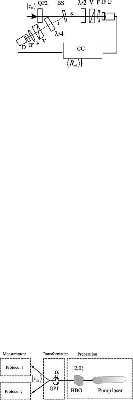
Unfortunately, the inverse matrix does not always exist. To simplify the problem we put only a single wave plate with ®xed optical thickness sds = p / 2 , di = p / 4d and ®xed orientation xs , ui in each channel of the Brown-Twiss scheme. In order to make sure the inverse matrix exists one needs to maximize the determinant of the matrix T over the orientations of the plates xs , ui. After accomplishing this procedure we obtain xs < −28.5°, ui < 19° (Fig. 4).
Instead of ®nding the links between the harmonics and moments, there is a more elegant method to reconstruct the quantum state using the second protocol (see Sec. III D). This method is considered in the present work.
B. Experimental implementation: Protocol 1
The experimental setup for the quantum tomography of qutrits using protocol 1 is shown in Fig. 5. The preparation block includes a 2-mm BBO crystal with either type-I or type-II degenerate and collinear phase matching, which is
FIG. 4. Measurement block for protocol 2. An additional control quartz plate sQP2d serves as the state ucinl tomography transformer. Only a single wave plate is introduced in each channel.
pumped with cw argon laser operated at 351 nm wavelength. In the case of type-II phase matching, an additional quartz compensator is introduced right after the crystal. The state C3 = u0 , 2l (for type I) or C2 = u1 , 1l (for type II) generated in the crystal is fed to the transformation block. This block consists of the quartz plate with ®xed optical thickness d = 0.9046 and variable orientation a. So the state, which is to be measured, is determined by the parameter a. The measurement block is a Brown-Twiss scheme equipped with polarization ®lters placed in both arms (Fig. 3). Pulses coming from a couple of single-photon modules (EG&G SPCMAQR) were fed to the counter through a standard time-to- amplitude converter.
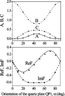
In our experiments the exposure time for measuring each moment is 5 sec. This time is an important experimental parameter. Each measurement consists of 30 runs, after which the scheme is reset. Namely each measurement is performed by setting the angles of wave plates xj and uj in both arms according to the tomographic protocol (Table I). After 30 runs, a new set of angles is selected and the next moment is measured in the same way. The output data of the setup are the mean coincidence counting rates. Examples of behavior for some moments sA , B , C , Re F , Im Fd versus the orientation of the plate QP1 are plotted in Fig. 6.
C. Experimental implementation: Protocol 2
For the second method we used Ti : Sa laser with pulse duration about 250 fsec, operating at 800 nm. After frequency doubling, the UV radiation with 400 nm wavelength was sent into the same setup as described above. For this protocol we used 2-mm BBO crystal cut for collinear degen-
FIG. 5. Scheme of qutrits tomograph, consisting of three blocks. Preparation block includes pump laser(s) and nonlinear crystal(s). Transformation block is the quartz plate sQP1d which orientation angle a determines the ®nal state to be measured. The measurement block depends on the protocol to be used (see Figs. 3 and 4).
042303-7
BOGDANOV et al.
FIG. 6. Some components of the matrix K4 versus the orientation of the quartz plate QP1. Different angles of the plate correspond to different states sent to the measurement block. The plot at
the |
top |
corresponds to measured |
real moments A (squares), B |
|
(circles), |
and C |
(triangles) and |
theoretical predictions As− d , |
|
Bs−− |
d , and Cs− ° − |
d. The plot at the bottom shows measured com- |
||
plex moment Re F (squares) and Im F (triangles), and theoretical predictions Re F (short-dashed line) and Im F (long-dashed line).
erate type-I phase matching. A quartz plate with the optical thickness d = 0.656 is placed after the BBO crystal to prepare the qutrit state to be measured. The measurement part of the setup was slightly changed (Fig. 4). An additional control quartz plate introduced in front of the beam splitter accomplishes the protocol. Its orientation angle m is a parameter de®ning the measurement process. The control plate is rotated with 5° steps from 0 up to 360° so that protocol 2 consists of 72 measurements. Each arm of the Brown-Twiss scheme contains either a quarteror half-wave plate with ®xed orientation. The orientations are x1 = 18.8° for the quarter-wave plate in the ®rst channel and u2 = −28.5° for the half-wave plate in the second channel. Protocol 2 is easier to implement since only a single parameter m is changed whereas four x1,2 , u1,2 parameters are varied in protocol 1. In perspective, this kind of protocol allows one to automate the quantum tomography procedure: the control plate can be rotated continuously and reconstruction of the quantum state can be based on analysis of coincidence rates corresponding to the respective values of mi si = 1 , . . . , 72d.
D. Statistical reconstruction of biphoton-®eld qutrits from the outcomes of mutually complementary measurements
Each of the nine processes from protocol 1 as well as of the 72 processes from protocol 2 is described by its amplitude Mn. From the statistical point of view, the squared modulus of the process amplitude speci®es the intensity of the event generation:
PHYSICAL REVIEW A 70, 042303 (2004)
Rn = Mn*Mn. |
s20d |
The considered processes are examples of mutually complementary sets of measurements in the sense of Bohr's complementarity principle. The event-generation intensities Rn for both protocols are the main quantities accessible from the measurement. Making the bridge between statistical and physical description of the process the quantities Rn coincide with the fourth moments in the ®eld introduced above in Eq. (19). Their dimension is the frequency unit (Hz). The number of events occurring within any given time interval obeys the Poisson distribution. Therefore, the quantities Rn specify the intensities of the corresponding mutually complementary Poisson processes and serve as estimates of the Poisson parameters ln (see below).
Although the amplitudes of the processes cannot be measured directly, they are of the greatest interest as these quantities describe fundamental relationships in quantum physics. It follows from the superposition principle that the amplitudes are linearly related to the state-vector components. So the main purpose of quantum tomography is the reproduction of the amplitudes and state vectors, which are hidden from direct observation.
The linear transformation of the state vector c = hc1 , c2 , c3j into the amplitude of the process M is described by a certain matrix X. For example, considering the ®rst protocol this matrix can be easily obtained from Table I (last column in Table I):
|
1 |
1/Î |
|
|
0 |
|
|
|
|
|
|
|
0 |
|
|
2 |
|
|
||||
|
2 |
|
|
|
|
|
|
|
|
|
|
|
||||||||||
|
0 |
|
|
1/2 |
|
|
|
|
|
|
|
0 |
|
|
|
|
||||||
|
0 |
|
|
0 |
|
|
|
|
|
|
|
1/Î |
|
|
|
|
||||||
|
|
|
|
|
|
|
|
|
|
2 |
|
|
||||||||||
|
0 |
|
|
|
1/s2Î |
|
|
|
d |
− i/2 |
|
|
||||||||||
|
|
|
2 |
|
|
|||||||||||||||||
|
0 |
|
|
|
1/s2Î |
|
|
|
d |
− 1/2 |
|
s21d |
||||||||||
X = |
|
|
2 |
. |
||||||||||||||||||
|
1/2 |
|
|
− 1/ s2Î |
|
|
d |
0 |
|
|
|
|
||||||||||
|
|
2 |
|
|
|
|
||||||||||||||||
|
1/2 |
|
|
− i/s2Î |
|
d |
0 |
|
|
|
|
|||||||||||
|
|
2 |
|
|
|
|
||||||||||||||||
|
|
|
|
|
|
|
|
|
|
|
|
|
|
|
|
|
|
|||||
|
|
|
|
|
|
|
|
|
|
|
|
|
|
|
|
|
|
|
|
|
|
|
042303-8

STATISTICAL RECONSTRUCTION OF QUTRITS
l = Frlss/2d rlsi/4d |
1 |
G. |
|
Î2 srlss/2d tlsi/4d + rlsi/4d tlss/2d d tlss/2d tlsi/4d |
s23d |
The unitary matrix G is de®ned by the control plate according to Eqs. (7) and (8), with a replacement a !m, where m is the control plate orientation (it takes 72 values from 0° to 355° ). We chose the control plate to be a quarter-wave plate, so d = p / 4. Finally,
G = Gsmid, i = 1,2, . . . ,72. |
s24d |
Each row of the instrumental matrix X (72 rows, 3 columns) is de®ned by the product of the row l (which is the same for any process) and the matrix G (which is de®ned by the control plate orientation angle):
Xi = lGsmid, i = 1,2, . . . ,72, |
s25d |
where Xi is the ith row of the matrix X.
IV. METHODS OF QUANTUM-STATE RECONSTRUCTION
In the simplest case the density matrix can be estimated directly from the measurements. Since the set of experimental data is limited in this case, the reconstructed density matrix may have nonphysical properties like negative eigenvalues. But in the general case of s-dimensional systems the problem of density matrix reconstruction using the direct results of measurements cannot be solved since the corresponding inverse problem is ill posed.
When analyzing the experimental data, we use the socalled root estimator of quantum states [17]. This approach is designed specially for the analysis of mutually complementary measurements (in the sense of Bohr's complementarity principle). The advantage of this approach consists of the possibility of reconstructing states in a high-dimensional Hilbert space and reaching the accuracy of reconstruction of an unknown quantum state close to its fundamental limit. Below we consider two methods of quantum-state root estimation that give similar results. They are the least-squares method (LSM) and maximum-likelihood method (MLM).
A. Least-squares method
In statistical terms, Eq. (22) is a linear regression equation. A distinctive feature of the problem is that only the absolute value of the process amplitude M is measured in the experiment. The estimate of the absolute value of the amplitude is given by the square root of the corresponding experimentally measured coincidence rate:
uMnu |
expt |
Î |
|
|
s26d |
|
|
||||
|
= kn/t, |
||||
where kn is the number of events (coincidences) detected in the nth process during the measurement time t.
It is worth noting that, by the action of the root-square procedure on a Poissonian random value, one gets the random variable with a uniform varianceÐi.e., at the variance stabilization [38]. Note also, since we do not deal with event probabilities but with their rates or intensities, it is convenient to use un-normalized state vectors. These vectors allow the coincidence counting rate (event-generation intensities)
PHYSICAL REVIEW A 70, 042303 (2004)
to be derived directly from Eqs. (20) and (22) without introducing coef®cients related to the biphoton generation rate, detector ef®ciencies, etc. The dimensionality of the vector state obtained in such a way is 1 / Îtime. The ®nal state vector obtained by the reconstruction procedure, nevertheless,
should be normalized to unity.
Assuming that the variances of different uMnuexpt are independent and identical, one can apply the standard leastsquares estimate to Eq. (22) [39]:
c = sX²Xd−1 X²M . |
s27d |
Unlike the traditional least-squares method, Eq. (27) cannot be used for an explicit estimation of the state vector c, be-
cause it is to be solved by the iteration method. The absolute value of M is known from the experiment suMnu = uMnuexptd.
We assume that the phase of vector Xc at the ith iteration step determines the phase of the vector M at the si + 1dth step. In other words, the phase is determined by the iteration procedure.
It turns out that, for the Gaussian approximation of Poisson's quantities, this least-squares estimate coincides with a more exact and rigorous maximum-likelihood estimate considered below.
B. Maximum-likelihood method
The likelihood function is de®ned by the product of Poissonian probabilities:
L = p slitidki e− liti , |
s28d |
|
i |
ki! |
|
where ki is the number of coincidences observed in the ith process during the measurement time ti, and li are the unknown theoretical event-generation intensities (expected number of coincidences proportional to the moments in the ®eld), whose estimation is the subject of this section.
The logarithm of the likelihood function is, if we omit an insigni®cant constant,
ln L = o fkilnslitid − litig. |
s29d |
i |
|
Let us introduce the matrices with the elements de®ned by the following formulas:
|
Ijs = o tiXi*jXis , |
s30d |
||
|
|
|
i |
|
Jjs = o |
ki |
Xi*jXis, j,s = 1,2,3. |
s31d |
|
|
||||
i |
li |
|
||
The matrix I is determined from the experimental protocol and, thus, is known a priori (before the experiment). This is the Hermitian matrix of Fisher's information. The matrix J is determined by the experimental values of ki and by the unknown event-generation intensities li. This is the empirical matrix of Fisher's information (see also the Appendix).
In terms of these matrices, the condition for the extremum of the function (29) can be written as
042303-9

BOGDANOV et al. |
PHYSICAL REVIEW A 70, 042303 (2004) |
TABLE II. Results of the state reconstruction. The left column indicates the orientation of the quartz plate QP1, determining the state to be measured. Values of the optical thickness of QP1 are d = 0.656 for the pulsed regime (protocols 1 and 2) and d = 0.9046 for the cw regime (protocol 1). Theoretical state vectors are placed in the right column. The table contains the amplitudes of the reconstructed states sc1 , c2 , c3d as well as their ®delities, calculated by least-squares (LSM) and maximum-likelihood (MLM) methods.
|
|
|
Pulsed regime, d = 0.656, protocol 1 |
|
|
|
|||
a |
Fidelity |
|
State vector: experiment |
|
State vector: theory |
||||
|
LSM |
MLM |
LSM |
|
MLM |
|
sc1 , c2 , c3dtheory |
|
|
0° |
0.99981 |
0.99979 |
−0.0046 + 0.0040 i |
−0.0065 + 0.0057 i |
0 |
|
|||
|
|
|
−0.0050 − 0.0115 |
i |
−0.0053 − 0.0102 |
i |
0 |
|
|
|
|
|
0.9999 |
|
0.9999 |
|
1 |
|
|
40° |
0.9989 |
0.9989 |
−0.3669 − 0.0691 |
i |
−0.3669 − 0.0687 |
i |
−0.3482 − 0.0948 |
i |
|
|
|
|
−0.0657 + 0.6814 i |
−0.0653 + 0.6815 i |
−0.0900 + 0.6732 i |
||||
|
|
|
0.6261 |
|
0.6261 |
|
0.6392 |
|
|
80° |
0.9993 |
0.9993 |
−0.0088 + 0.0439 i |
−0.0091 + 0.0439 i |
−0.0136 + 0.0413 i |
||||
|
|
|
0.1691 |
+ 0.2587i |
|
0.1697 + 0.259i |
|
0.1691 + 0.2338i |
|
|
|
|
0.9500 |
|
0.9498 |
|
0.9565 |
|
|
|
|
|
Pulsed regime, d = 0.656, protocol 2 |
|
|
|
|||
0° |
0.99846 |
0.99847 |
−0.0071 − 0.0135 |
i |
−0.0072 − 0.0135 |
i |
0 |
|
|
|
|
|
0.0359 + 0.0046i |
|
0.0357 + 0.0046i |
|
0 |
|
|
|
|
|
0.9992 |
|
0.9992 |
|
1 |
|
|
40° |
0.9991 |
0.9991 |
−0.3442 − 0.1139 |
i |
−0.3444 − 0.1142 |
i |
−0.3482 − 0.0948 |
i |
|
|
|
|
−0.0987 + 0.6546 i |
−0.0990 + 0.6545 i |
−0.0900 + 0.6732 i |
||||
|
|
|
0.6560 |
|
0.6559 |
|
0.6392 |
|
|
80° |
0.9981 |
0.9981 |
−0.0093 + 0.0430 i |
−0.0094 + 0.0430 i |
−0.0136 + 0.0413 i |
||||
|
|
|
0.2122 + 0.2408i |
|
0.2121 + 0.2408i |
|
0.1691 + 0.2338i |
|
|
|
|
|
0.9461 |
|
0.9461 |
|
0.9565 |
|
|
|
|
|
cw regime, d = 0.9046, protocol 1 |
|
|
|
|||
0° |
0.99325 |
0.99313 |
−0.0030 − 0.0512 |
i |
−0.0028 − 0.0514 |
i |
0 |
|
|
|
|
|
0.9966 |
|
0.9966 |
|
1 |
|
|
|
|
|
−0.0015 − 0.0642 |
i |
−0.0013 − 0.0649 |
i |
0 |
|
|
60° |
0.9886 |
0.9799 |
0.7236 |
|
0.7244 |
|
0.7052 |
|
|
|
|
|
0.1165 − 0.1231 i |
|
0.1245 − 0.1210 i |
|
0.0392 − 0.0616 i |
|
|
|
|
|
0.2792 + 0.6080i |
|
0.1694 + 0.6453i |
|
0.2990 + 0.6387i |
|
|
|
|
|
|
|
|
|
|
|
|
|
|
|
|
|
|
|
|
|
|
Ic = Jc. |
s32d |
o ki = o slitid. |
s34d |
|
|
|
i |
i |
|
Hence, it follows that
I−1 Jc = c. |
s33d |
The latest relationship is known as the likelihood equation. This is a nonlinear equation, because li depends on the unknown state vector c. Because of the simple quasilinear structure, this equation can easily be solved by the iteration method [17]. The quasi-identity operator I−1 J acts as the identical operator upon only a single vector in the Hilbert spaceÐnamely, on the vector corresponding to the solution of Eq. (33) and representing the maximum possible likelihood estimate for the state vector. The condition for the existence of the matrix I−1 is a condition imposed on the initial experimental protocol. The resulting set of equations automatically includes the normalization condition, which is written as
This condition implies that, for all processes, the total number of detected events is equal to the sum of the products of event detection frequencies during the measurement time.
C. Analysis of the experimental data
1. Pure-state reconstruction
The examples of qutrit state reconstruction using both the least-squares and maximum-likelihood methods are given in Table II.
The value of the ®delity parameter F is de®ned as
F = ukctheoryucexptlu2 . |
s35d |
It gives a conventional measure of the correspondence between the theoretical and experimental state vectors.
042303-10