PRA42303

STATISTICAL RECONSTRUCTION OF QUTRITS

FIG. 7. Fidelity dependence on the sample size. Mean values and standard deviations corresponding to the sample volumes f = 0.01 , 0.04 , 0.1 , 0.25 , 0.5 , 1.0.

The dependence of ®delity on the amount of experimental data obtained is shown in Fig. 7. This ®gure shows the ®delity achieved in the experiment in comparison with the theoretical range (see the Appendix for more details). The lower boundary corresponds to 5% quantile of statistical distribution, while the upper to 95% quantile. It is clearly seen that the ®delity value achieved experimentally for a small volume of experimental data is completely within the limits of the theoretical range, while it goes out for a higher volume. Such behavior of ®delity is due to the existence of two different error types arising under the reconstruction of quantum states. Let us call them statistical and instrumental errors, respectively. The statistical errors are caused by a ®nite number of quantum system representatives to be measured. As the measurement time increases, the information about the quantum state of interest progressively increases (see the Appendix). Accordingly, the statistical error becomes smaller. The instrumental errors are caused by the researcher's incomplete knowledge of the system; i.e., more exact information exists, in principle, but it is inaccessible to the experimenter. Thus, a comparison between the state reconstruction result and the fundamental statistical level of accuracy can serve as a guide for the parameter adjustment of the setup.

Thus, for a small volume of experimental data, statistical errors prevail, whereas for large sample sizes, the setting errors and the instability of protocol parameters dominate. The number of events at which the statistical error becomes smaller than the instrumental error can be called the coherence volume. Numerically the coherence volume can be estimated as the intersection point between the experimental ®delity and the lower theoretical ®delity curve. In our case this value is about 25 000 ± 30 000 events. Starting approximately from this value, ®delity is reaching saturation and further growth of experimental data volume does not lead to an increase in the precision of quantum system estimation.

Figure 7 relates to the state de®ned by the orientation angle of the quartz plate QP1 a = 50° (for protocol 2). To plot Fig. 7 we used the following technique for passing from full-volume experiment to a partial-volume experiment. Let us consider the parameter 0 , f ø 1, which characterizes the volume of experimental data. Suppose that f = 1 for a fullvolume experiment. A partial-volume experiment may be in-

PHYSICAL REVIEW A 70, 042303 (2004)

FIG. 8. Informational x2 criterion for small sample sizes: sample size = 4400.

tn. Hence, performing a single full-volume experiment means providing with a large (practically in®nite) number of partialvolume experiments.

For a given volume of experimental data f each event from the full-volume experiment is picked up with the probability f and rejected with the probability 1 − f. Due to the presence of statistical ¯uctuations, the equation for the number of observations, knst8nd = fknstnd, is violated. Therefore a unique estimate of the state vector corresponds to every partial-volume experiment. Figure 7 shows mean values and

The results of informational ®delity research, introduced in the Appendix, are shown in Figs. 8 and 9. These ®gures correspond to the same data set as shown in Fig. 7. The distribution density of informational ®delity for a small (compared to the coherence volume) sample size closely agrees with the theoretical result given by Eq. (A14) (see Fig. 8). In this case the instrumental error is negligibly small compared to the statistical one. When the sample volume is close to the coherence volume (Fig. 9) the in¯uence of instrumental and statistical errors is about equal. In other

FIG. 9. Informational x2 criterion for large sample sizes: sample size = 27 750. The disagreement between observations and theoretical curve for large sample sizes is due to the instrumental error.

BOGDANOV et al.

TABLE III. Example of the mixture separation using quasiBayesian algorithm for the given state. cw regime, protocol 1.

Fidelity = 0.9916

words, the informational losses caused by averaging over instrumental errors are approximately equal to the losses caused by statistical ones. Finally, if the sample size is greater than the coherence volume, instrumental errors predominate. It means that the statistical informational errors are negligibly small compared to the instrumental ones.

2. Mixture separation algorithm

Let us describe the algorithm for reconstructing a twocomponent mixed state. This algorithm can be easily generalized to an arbitrary number of components.

The total number of events observed in every process is divided between the components proportional to the intensity:

At a certain iteration step, let us represent kn as a sum of

For each component, we can obtain the estimates for the state vector, amplitudes, and intensity of the processes according to the method of pure-state analysis described in the previous section. Since we get new intensity estimates, let us again split the total number of events in every process proportionally to the intensities of the components. In such a way, a new iteration is formed and the whole procedure is repeated. The described process is called quasi-Bayesian algorithm [17].

As a result, the iteration process converges to some (nonnormalized) components cs1d and cs2d. Thus, the mixture separation algorithm reduces to numerous estimations of pure components according to the simple algorithm described above in Sec. IV B. As a result of the whole algorithm execution, the estimate for the density matrix of the mixture appears:

PHYSICAL REVIEW A 70, 042303 (2004)

TABLE IV. Analysis of the principal components of the density matrix for the state (41) and (42): numerical simulation.

r

r ! Trsrd . s39d

The last procedure is normalization of the density matrix. A remarkable feature of the algorithm is that according to

numerical calculations, independent of zero-approximation selection of the mixture components, the resulting density matrix r is always the same. Of course, the components cs1d and cs2d are different for the random selection of the zero approximation.

The mixed-state reconstruction accuracy is described by the following ®delity:

where rs0d and r are the exact and reconstructed density matrices, respectively. For a pure state fr2 = r , srs0dd2 = rs0dg ®- delity (40) converts to Eq. (35).

Actually in the present work we did not intend to generate a given mixed state of qutrits in experiment; it will be done later [40]. Nevertheless, applying the described algorithm to the data we can check whether the state produced in our system is pure. For example, consider the case when the state C2 = u1 , 1l is fed to the quartz plate QP1 (see Table II). This state is the most interesting to be tested, since uH , Vl and uV , Hl are distinguishable due to the polarization dispersion in BBO crystal. Namely, extraordinarily polarized photons sHd propagate faster than ordinary sVd ones in the crystal. Therefore a group velocity compensator has to be used for making them indistinguishable [41]. Nonperfect compensation (we reached 95% visibility for polarization interference) is the main reason why the ®delity reconstruction for these states is not so high. The results of applying quasi-Bayesian algorithm to the reconstructed state are in Table III. We chose the state corresponding to the angle a = 30°. It is clearly seen that the weight of the ®rst principal component is much greater than that of the second one. Doing the same procedure with the C1 = u2 , 0l initial state, we have checked that the estimator for a pure-state vector is extremely close to the estimator of the major density matrix component.

STATISTICAL RECONSTRUCTION OF QUTRITS

To illustrate the quasi-Bayesian approach, let us consider a result of reconstruction for a two-component mixture using protocol 1. Suppose one has a mixture of two pure states prepared from u2 , 0l by quartz plates QP18 and QP19 oriented at angles a = −30° and a = 50°, respectively. Let the

PHYSICAL REVIEW A 70, 042303 (2004)

optical thickness of both plates be d = 0.656. Ten thousand events were generated (on the average) for every component. The theoretical density matrix for the mixed state under consideration is

The reconstructed matrix ®delity is F = 0.999 431. An analysis of the principal components of density matrix is given in Table IV.

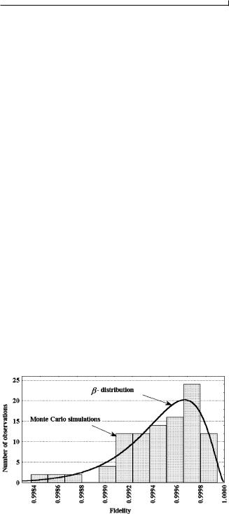
This example shows a reasonably high accuracy of mixed-state reconstruction. The statistical properties of the proposed algorithm were studied by means of the Monte Carlo method. One hundred numerical experiments were conducted similar to the one described above. To verify the reliability, the solution was found twice for each experiment (with random zero-approximation selection). The solutions appeared to be equal for all cases (within a negligibly small computational error). The obtained statistical ®delity distribution is shown in Fig. 10. Numerical research shows that the ®delity distribution density is well described by the b distribution.

V. CONCLUSION

The procedure of quantum-state measurement for a threestate optical system formed by a frequency and spatially de-

FIG. 10. Simulation of the ®delity between theoretical and reconstructed density matrices in a mixture separation problem. Here 100 numerical experiments of 20 000 events per each (on the average) were made.

generate two-photon ®eld has been considered in this work. A method of statistical estimation of the quantum state through solving the likelihood equation and examining the statistical properties of the resulting estimates has been developed. Based on the experimental data (fourth-order moments in the ®eld) and the root method of estimating quantum states, the initial wave function of qutrits has been reconstructed.

Experimental data analysis is based on representing the event-generation intensity for each one of mutually complementary quantum processes as a squared module of some amplitude. A complete set of measured processes amplitudes can be compactly described using the instrumental matrix. In the framework of the formalism of a process amplitude one can apply effective tools for the quantum state reconstruction: least-squares and maximum-likelihood methods.

The developed analysis tools provide the means of quantum-state reconstruction from the experimental data with high accuracy and reliability. The estimate accuracy is determined by the concurrence of two types of errors: statistical ones and instrumental ones. For smaller sample sizes statistical errors are dominant, while for greater ones instrumental errors dominate.

Instrumental errors lead to ®delity saturation at less than unity level. In the present work, ®delity for most of performed experiments (more than 20) exceeded a level of 0.995. For many cases the level of 0.9998 was achieved.

ACKNOWLEDGMENTS

Useful discussions with A. Burlakov, A. Ekert, B. Englert, D. Kazlikowski, and A. Lamas-Linares are gratefully acknowledged. This work was supported in part by the Russian Foundation of Basic Research (Project Nos. 03-02-16444 and 02-02-16843), National University of Singapore Program WBS (Project No. R-144-000-100-425), and the National University of Singapore's Eastern Europe Research Scientist and Student Programme. One of us (L.K.) acknowledges support from a INTAS-YS grant (No. 03-55-1971).

BOGDANOV et al.

APPENDIX: STATISTICAL FLUCTUATIONS

OF THE STATE VECTOR

As was already mentioned above, an un-normalized state vector provides the most complete information about a quantum system. The use of an un-normalized vector allows us to remove an interaction constant in Eq. (22). The norm of the vector c, obtained as a result of quantum system reconstruction, provides one with information about the total intensity of all the processes considered in the experiment. However, the ¯uctuations of the quantum state (and norm ¯uctuations, in particular) in a normally functioning quantum information system should be within a certain range de®ned by the statistical theory. The present section is devoted to this problem.

The practical signi®cance of accounting for statistical ¯uctuations in a quantum system relates to developing methods of estimation and control of the precision and stability of a quantum information system evolution, as well as methods of detecting external interception (Eve's attack on the quantum channel between Alice and Bob).

The estimate of the un-normalized state vector c, obtained by the maximum-likelihood principle, differs from the exact state vector cs0d by the random values dc = cs0d − c. Let us consider the statistical properties of the ¯uctuation vector dc by expansion of the log-likelihood function near a stationary point:

d ln L = − F21 sKsjdcsdcj + K*sjdc*s dc*j d + Isjdc*s dcjG.

sA1d

Together with the Hermitian matrix of the Fisher information I, Eq. (30), we de®ne the symmetric Fisher information matrix K, whose elements are de®ned by the following equation:

where Mn is the amplitude of the nth process. In the general case, K is a complex symmetric non-Hermitian matrix. From all possible types of ¯uctuations, let us pick out the so-called gauge ¯uctuations. In®nitesimal global gauge transformations of a state vector are as follows:

where « is an arbitrary small real number and s is the Hilbert space dimension.

Evidently, for gauge transformations, d ln L = 0. It means that two state vectors that differ by a gauge transformation are statistically equivalent; i.e., they have the same likelihood. Such vectors are physically equivalent since the global phase of the state vector is nonobservable. From a statistical point of view, the set of mutually complementing measurements should be chosen in such a way that for all other ¯uctuations (except gauge ¯uctuations) d ln L , 0. This inequality serves as the statistical completeness condition for the set of mutually complementing measurements.

PHYSICAL REVIEW A 70, 042303 (2004)

Let us derive some constructive criteria of the statistical completeness of measurements. The complex ¯uctuation vector dc is conveniently represented by a real vector of double length. After extracting the real and imaginary parts

In the particular case of qutrits ss = 3d this transition provides us with a six-component real vector instead of a threecomponent complex vector.

In the new representation, Eq. (A1), becomes

d ln L = − Hsjdjsdjj = − kdjuHudjl, sA5d

where matrix H is the ªcomplete information matrixº possessing the following block form:

The matrix H is real and symmetric. It is of double dimension, respectively, to the matrices I and K. For qutrits, I and K are 3 3 3 matrices, while H is 6 3 6.

Using matrix H it is easy to formulate the desired characteristic completeness condition for a mutually complementing set of measurements. For a set of measurements to be statistically complete, it is necessary and suf®cient that one and only one eigenvalue of the complete information matrix H is equal to zero, while the other ones are strictly positive.

We would like to stress that checking the condition one not only veri®es the statistical completeness of a measurement protocol, but also ensures that the obtained extremum is of maximum likelihood.

An eigenvector that has eigenvalue equal to zero corresponds to gauge ¯uctuation direction. Such ¯uctuations do not have a physical meaning as stated above. Eigenvectors corresponding to the other eigenvalues specify the direction of ¯uctuations in the Hilbert space.

The principal ¯uctuation variance is

where hj is the eigenvalue of the information matrix H, corresponding to the jth principal direction.

The most critical direction in the Hilbert space is the one with the maximum variance s2j , while the corresponding eigenvalue hj is accordingly minimal. Knowledge of the numerical dependence of statistical ¯uctuations allows one to estimate distributions of various statistical characteristics.

The important information criterion that speci®es the general possible level of statistical ¯uctuations in a quantum information system is the x2 criterion. It can be expressed as

PHYSICAL REVIEW A 70, 042303 (2004)

Relation (A11) describes the distribution of relative information ¯uctuations. It shows that the relative information uncertainty of a quantum state decreases with the number of observations as 1 / n.

The mean value of relative information ¯uctuations is

The information ®delity may be introduced as a measure of correspondence between the theoretical state vector and its estimate:

Correspondingly, the value 1 − FH is the information loss. The convenience of FH relies on its simpler statistical

properties compared to the conventional ®delity F. For a system where statistical ¯uctuations dominate, ®delity is a

where x2s2s − 1 d is a random value of x2 type with 2s − 1 degrees of freedom.

Information ®delity asymptotically tends to unity when the sample size is growing up. Complementary to statistical ¯uctuations noise leads to a decrease in the informational ®delity level compared to the theoretical level (A14).