0303014

Yu.I. Bogdanov LANL Report quant-ph/0303014

Root Estimator of Quantum States

Yu. I. Bogdanov

OAO "Angstrem", Moscow, Russia

E-mail: bogdanov@angstrem.ru

Abstract

The root estimator of quantum states based on the expansion of the psi function in terms of system eigenfunctions followed by estimating the expansion coefficients by the maximum likelihood method is considered. In order to provide statistical completeness of the analysis, it is necessary to perform measurements in mutually complementing experiments (according to the Bohr terminology). Estimation of quantum states by the results of coordinate, momentum, and polarization (spin) measurements is considered. The maximum likelihood technique and likelihood equation are generalized in order to analyze quantum mechanical experiments. The Fisher information matrix and covariance matrix are considered for a quantum statistical ensemble. The constraints on the energy are shown to result in high-frequency noise reduction in the reconstructed state vector. Informational aspects of the problem of division a mixture are studied and a special (quasiBayesian) algorithm for solving this problem is proposed. It is shown that the requirement for the expansion to be of a root kind can be considered as a quantization condition making it possible to choose systems described by quantum mechanics from all statistical models consistent, on average, with the laws of classical mechanics.

Introduction.

In the previous paper (“Quantum Mechanical View of Mathematical Statistics” quantph/0303013- hereafter, Paper 1), is has been shown that the root density estimator, based on the introducing an object similar to the psi function in quantum mechanics into mathematical statistics, is an effective tool of statistical data analysis. In this paper, we will show that in problems of estimating of quantum states, the root estimators are at least of the same importance as in the problems of classical statistical analysis.

Methodologically, the method considered here essentially differs from other well known methods for estimating quantum states that arise from applying the methods of classical tomography and classical statistics to quantum problems [1-3]. The quantum analogue of the distribution density is the density matrix and the corresponding Wigner distribution function. Therefore, the methods developed so far have been aimed at reconstructing the aforementioned objects in analogy with the methods of classical tomography (this resulted in the term “quantum tomography”) [4].

In [5], a quantum tomography technique on the basis of the Radon transformation of the Wigner function was proposed. The estimation of quantum states by the method of least squares was considered in [6]. The maximum likelihood technique was first presented in [7,8]. The version of the maximum likelihood method providing fulfillment of basic conditions imposed of the density matrix (hermicity, nonnegative definiteness, and trace of matrix equal to unity) was given in [9,10]. Characteristic features of all these methods are rapidly increasing calculation complexity with increasing number of parameters to be estimated and ill-posedness of the corresponding algorithms, not allowing one to find correct stable solutions.

The orientation toward reconstructing the density matrix overshadows the problem of estimating more fundamental object of quantum theory, i.e., the state vector (psi function). Formally, the states described by the psi function are particular cases of those described by the density matrix. On the other hand, this is the very special case that corresponds to fundamental laws in Nature and is related to the situation when the state described by a large number of unknown parameters may be stable and estimated up to the maximum possible accuracy.

1

Yu.I. Bogdanov LANL Report quant-ph/0303014

In Sec. 1, the problem of estimating quantum states is considered in the framework of the mutually complementing measurements (Bohr [11]). The likelihood equation and statistical properties of estimated parameters are studied.

In Sec. 2, the maximum likelihood method is generalized on the case when, along with the condition on the norm of a state, additional constraint on energy is introduced. The latter restriction allows one to suppress noise corresponding to the high-frequency range of the spectrum of a quantum state.

In Sec. 3, the problem of reconstructing the spin state is briefly considered. In the nonrelativistic approximation, the coordinate and spin wave functions are factorized; therefore, the corresponding problems of reconstructing the states can be considered independently in the same approximation.

The mixture separation problem is considered in Sec. 4. It is shown that from the information standpoint it is purposefully to divide initial data into uniform (pure) sets and perform independent estimation of the state vector for each set. A quasiBayesian self-consistent algorithm for solving this problem is proposed.

In Sec. 5, it is shown that the root expansion basis following from quantum mechanics is preferable to any other set of orthonormal functions, since the classical mechanical equations are satisfied for averaged quantities according to the Ehrenfest theorems. Thus, the requirement for the probability density to be of the root form plays a role of the quantization condition.

1. Phase Role. Statistical Analysis of Mutually Complementing Experiments. Statistical Inverse Problem in Quantum Mechanics.

We have defined in the Paper.1 the psi function as a complex-valued function with the squared absolute value equal to the probability density. From this point of view, any psi function

can be determined up to arbitrary phase factor exp(iS(x)). In particular, the psi function can be

chosen real-valued. For instance, in estimating the psi function in a histogram basis, the phases of amplitudes (4.2) of the Paper.1, which have been chosen equal to zero, could be arbitrary.

At the same time, from the physical standpoint, the phase of psi function is not redundant. The psi function becomes essentially complex valued function in analysis of mutually complementing (according to Bohr) experiments with micro objects [11].

According to quantum mechanics, experimental study of statistical ensemble in coordinate space is incomplete and has to be completed by study of the same ensemble in another (canonically conjugate, namely, momentum) space. Note that measurements of ensemble parameters in canonically conjugate spaces (e.g., coordinate and momentum spaces) cannot be realized in the same experimental setup.

The uncertainty relation implies that the two-dimensional density in phase space

separately in mutually complementing experiments and then combined by introducing the psi function. We will consider the so-called sharp measurements resulting in collapse of the wave function (for unsharp measurements, see [12]).

The coordinate-space and momentum-space psi functions are related to each other by the Fourier transform ( h =1)

2

Yu.I. Bogdanov LANL Report quant-ph/0303014

Consider a problem of estimating an unknown psi function (ψ(x) or ψ~(p)) by

experimental data observed both in coordinate and momentum spaces. We will refer to this problem as an statistical inverse problem of quantum mechanics (do not confuse it with an inverse problem in the scattering theory). The predictions of quantum mechanics are considered as a direct problem. Thus, we consider quantum mechanics as a stochastic theory, i.e., a theory describing statistical (frequency) properties of experiments with random events. However, quantum mechanics is a special stochastic theory, since one has to perform mutually complementing experiments (spacetime description has to be completed by momentum-energy one) to get statistically full description of a population (ensemble). In order for various representations to be mutually consistent, the theory should be expressed in terms of probability amplitude rather than probabilities themselves.

A simplified approach to the inverse statistical problem, which will be exemplified by

( ) ~( )

P x and P p have

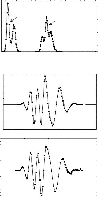
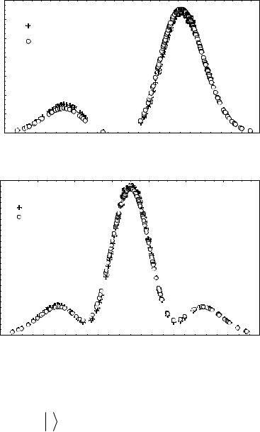
already been found (e.g., by histogram estimation). It is required to approximate the psi function for a statistical ensemble. Figure 1 shows the comparison between exact densities that could be calculated if the psi function of an ensemble is known (solid line), and histogram estimators obtained in mutually complementing experiments. In each experiment, the sample size is 10000 points. In Fig. 2, the exact psi function is compared to that estimated by samples. The solution was found by iteration procedure of adjusting the phase of psi function in coordinate and momentum

representations. In zero-order approximation ( (r = 0)), the phases were assumed to be zero. The

momentum-space phase in the r +1 approximation was determined by the Fourier transform of the psi function in the r approximation in the coordinate space and vice versa.

The histogram density estimator results in the discretization of distributions, and hence, natural use of the discrete Fourier transform instead of a continuous one.

Examples of mutually complementing experiments that are of importance from the physical point of view are diffraction patterns (for electrons, photons, and any other particles) in the nearfield zone (directly downstream of the diffraction aperture) and in the Fraunhofer zone (far from the diffraction aperture). The intensity distribution in the near-field zone corresponds to the coordinate probability distribution; and that in the Fraunhofer zone, the momentum distribution. The psi function estimated by these two distributions describes the wave field (amplitude and phase) directly at the diffraction aperture. The psi function dynamics described by the Schrödinger equation for particles and the Leontovich parabolic equation for light allows one to reconstruct the whole diffraction pattern (in particular, the Fresnel diffraction).

In the case of a particle subject to a given potential (e.g., an atomic electron) and moving in a finite region, the coordinate distribution is the distribution of the electron cloud, and the momentum distribution is detected in a thought experiment where the action of the potential abruptly stops and particles move freely to infinity.

In quantum computing, the measurement of the state of a quantum register corresponds to the measurement in coordinate space; and the measurement of the register state after performing the discrete Fourier transform, the measurement in momentum space. A quantum register involving

n qubits can be in 2n states; and correspondingly, the same number of complex parameters is to be estimated. Thus, exponentially large number of measurements of identical registers is required

From the standpoint of quantum mechanics, the formula (1.3) implies that the same quantity, namely, the mean square momentum, is defined in two different representations (coordinate and momentum). This quantity has a simple form in the momentum representation, whereas in the coordinate representation, it is rather complex characteristic of distribution shape

3

Yu.I. Bogdanov LANL Report quant-ph/0303014

(irregularity). The corresponding quantity is proportional to the Fisher information on the translation parameter of the distribution center.

Fig. 2 Comparison between exact psi function (solid line) and that estimated by a sample (dots).

The irregularity cannot be measured in the coordinate space in principle, since it refers to another (momentum) space. In other words, if there is no any information from the canonically conjugate space, the distribution irregularity in the initial space may turn out to be arbitrary high. Singular distributions used in probability theory can serve as density models with an infinite irregularity. From mathematical statistics, it is well-known that arbitrary large sample size does not allow one to determine whether the distribution under consideration is continuous or singular. This causes the ill-posedness of the inverse problem of the probability theory [13].

4

Yu.I. Bogdanov LANL Report quant-ph/0303014

Thus, from the standpoint of quantum mechanics, the ill-posedness of the classical problem of density estimation by a sample is due to lack of information from the canonically conjugate space. Regularization methods for inverse problem consist in excluding a priory strongly-irregular functions from consideration. This is equivalent to suppression of high momenta in the momentum space.

Let us turn now to more consistent description of the method for estimation of the state vector of a statistical ensemble on the basis of experimental data obtained in mutually complementing experiments. Consider corresponding generalization of the maximum likelihood principle and likelihood equation. To be specific, we will assume that corresponding experiments relate to coordinate and momentum spaces.

We define the likelihood function as

The maximum likelihood principle together with the normalization condition evidently results in the problem of maximization of the following functional:

By full analogy with calculations conducted in Sec.3 of the Paper.1, it can be proved that the

most likely state vector always corresponds to the eigenvalue of the R matrix (equal to sum of measurements).

The likelihood equation can be easily expressed in the form similar to (3.10) of the Paper.1:

The Fisher information matrix (prototype) is determined by the total information contained in mutually complementing experiments (compare to (1.5) and (1.6) of the Paper. 1):

5

Note that the factor of 4 is absent in (1.12) in contrast to the similar formula (1.6) of the

Paper.1. This is because of the fact that it is necessary to distinguish ψ(x) and ψ (x) as well as

c and c .

Consider the following simple transformation of a state vector that is of vital importance (global gauge transformation). It is reduced to multiplying the initial state vector by arbitrary phase

where α is arbitrary real number.

One can easily verify that the likelihood function is invariant against the gauge transformation (1.13). This implies that the state vector can be estimated by experimental data up to arbitrary phase factor. In other words, two state vectors that differ only in a phase factor describe the same statistical ensemble. The gauge invariance, of course, also manifests itself in theory, e.g., in the gauge invariance of the Schrödinger equation.

The variation of a state vector that corresponds to infinitesimal gauge transformation is

where α is a small real number.

Consider how the gauge invariance has to be taken into account in considering statistical

likelihood method from the true state vector characterizing the statistical ensemble.

In view of the gauge invariance, let us divide the variation of a state vector into two terms δc =δ1c +δ2c . The first term δ1c = iα c corresponds to gauge arbitrariness, and the second

one δ2c is a real physical fluctuation.

An algorithm of dividing of the variation into gauge and physical terms can be represented as follows. Let δc be arbitrary variation meeting the normalization condition. Then, (1.15) yields

Let us show that this gauge transformation provides minimization of the sum of squares of variation absolute values. Let (δc j )c j = iε . Having performed infinitesimal gauge transformation, we get the new variation

6

Evidently, the last expression has a minimum at α =ε .

Thus, the gauge transformation providing separation of the physical fluctuation from the

Here, we have dropped the subscript 2 assuming that the state vector variation is a physical fluctuation free of the gauge component).

Second, this transformation results in mean square minimization of possible variations of a state vector.

The inversion of the Fisher matrix yields the truncated covariance matrix (without zero component). Having calculated covariations with zero components in an explicit form, we finally find the expression for the total covariance matrix that is similar to (1.19) of the Paper.1:

The Fisher information matrix and covariance matrix are Hermitian. It is easy to see that the covariance matrix (1.23) satisfies the condition similar to (1.21) of the Paper.1:

By full analogy with the reasoning of Sec.1 of the Paper.1, it is readily seen that the matrix (1.23) is the only (up to a factor) Hermitian tensor of the second order that can be constructed from a state vector satisfying the normalization condition.

The formula (1.23) can be evidently written in the form

7

where U is the unitary matrix, and D is the diagonal matrix.

The diagonal of the D matrix has the only zero element (the corresponding eigenvector is

and their linear combinations form subspace that is orthogonal complement to a state vector).

The chi-square criterion determining whether the scalar product between the estimated and true vectors cc (0) is close to unity that is similar to (2.1) of the Paper. 1 is

Gaussian type and equal to half of the ordinary random chi-square of the number of the degrees of freedom doubled.

In terms of the density matrix, the expression (1.27) may be represented in the form

The chi-square criterion to test the homogeneity of two samples under consideration can be represented in two different forms:

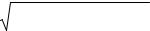
This method is illustrated in Fig. 3. In this figure, the density estimator is compared to the true densities in coordinate and momentum spaces.

8

Yu.I. Bogdanov LANL Report quant-ph/0303014

p

The sample of a size of n = m = 200 ( n + m = 400 ) was taken from a statistical

ensemble of harmonic oscillators with a state vector with three nonzero components ( s =3). The state of quantum register is determined by the psi function

Here, ni and mj are the number of measurements made in corresponding states. In the case under consideration, the likelihood equation similar to (1.10) has the form

9

Yu.I. Bogdanov LANL Report quant-ph/0303014

2. Constraint on the Energy

As it has been already noted, the estimation of a state vector is associated with the problem of suppressing high frequency terms in the Fourier series. In this section, we consider the regularization method based on the law of conservation of energy. Consider an ensemble of harmonic oscillators (although formal expressions are written in general case). Taking into account the normalization condition without any constraints on the energy, the terms may appear that make a negligible contribution to the norm but arbitrary high contribution to the energy. In order to suppress these terms, we propose to introduce both constraints on the norm and energy in the maximum likelihood method. The energy is readily estimated by the data of mutually complementing experiments.

It is worth noting that in the case of potentials with a finite number of discrete levels in quantum mechanics [14], the problem of truncating the series does not arise (if solutions bounded at infinity are considered).

We assume that the psi function is expanded in a series in terms of eigenfunctions of the

Here, Ei is the energy level corresponding to i -th state.

The mean energy corresponding to a statistical ensemble with a wave function ψ(x) is

Consider a problem of finding a maximum likelihood estimator of a state vector in view of a constraint on the energy and norm of the state vector. In energy basis, the problem is reduced to maximization of the following functional:

the same result representing the relationship between the Lagrange multipliers:

10