

electrodynamics / Companion to J.D. Jackson's Classical Electrodynamics 3rd ed. - R. Magyar
.pdfProblem 9.17
Treat the linear antenna of Problem 9.16 by the multi-pole expansion method.
Until further notice: the units in this problem are inconsistent. check them! a. Calculate the multi-pole moments (electric dipole, magnetic dipole, and electric quadrupole) exactly and in the long wavelength approximation.
For a linear antenna:
|
~ |
|
|
|
|
|
|
|
|
|
|
|
|
|
|
|
J(~r) = zˆ sin(kz)δ(x)δ(y)I0 |
|
|
|
|
|
|||||||||
Use the multi-pole expansion. |
|
|
|
|
|
|
|
|
|
|
|
||||
lim |
A~ ~x |
µ0 eikr |
|
( |
ik)n |
|
J~ ~x′ |
|
n |
|
~x′ |
|
ndV ′ |
||
|
|
|
|
|
|
|
|
|
|
||||||
4π r |
n |
|
−n! |
Z |
)( |
· |
) |
||||||||
kr→∞ |
( ) = |
|
( |
|
|
|
|||||||||
|
|
|
|
|
X |
|
|
|
|
|
|
|
|
|
|
For n=1 in the expansion, we find the electric dipole contribution:
~ |
µ0 eikr |
|
~ ′ |
|
′ |
|
µ0 eikr |
|
|
d |
′ |
|
′ |
|
||||
|
|
|
|
|
2 |
|
|
|||||||||||
A = |
|
|
|
Z |
J(~r |
)dV |
|
= |
|
|
|
zIˆ |
0 |
Z− d2 |
sin(kz |
)dz |
|
= 0 |
4π r |
|
4π r |
|
|||||||||||||||
When n=2 in the expansion, we get a term proportional to the integral of
~ ′
J (~n · ~r ). Using the vector identities, this can be rewritten in terms of the magnetic dipole and electric quadrapole contributions. The magnetic dipole contribution is:
|
|
|
|
A~ = − |
µ0 eikr ik |
Z (~r′ × J~(~r′)) × ~ndV ′ |
= 0 |
|
|
|
|
|
|
|
|
|
|
|||||||||||||||||||||||||||||||
|
|
|
|
4π |
|
|
|
r |
|
|
2 |
|
|
|
|
|
|
|
|
|
|
|
||||||||||||||||||||||||||
The electric quadrapole contribution is: |
|
|
|
|
|
|
|
|
|
|
|
|
|
|
|
|
|
|
|
|
|
|
|
|
|
|||||||||||||||||||||||
|
|
|
|
|
|
|
|
|
|
|
|
|
|
|
µ0 eikr ik |
|
|
|
|
|
|
|
|
|
|
|
|
|
|
|
|
|
|
|
|
|
|
|
|
|
||||||||
|
|
|
|
|
|
A~ = − |
|
|
|
|
|
|
Z |
|
(~n · ~r′)J~(~r′) + (~n · J~(~r′))~r′ |
dV ′ |
||||||||||||||||||||||||||||||||
|
|
|
|
|
4π |
r |
2 |
|||||||||||||||||||||||||||||||||||||||||
|
|
|
|
|
|
µ0 |
|
eikr |
|
ik |
|
|
|
|
|
|
d |
|
|
h |
|
|
|
|
|
|
|
|
|
|
|
|
|
|
|
|
|
i |
|
|
||||||||
|
= |
|
|
|
zIˆ 0 |
2 [z′ |
cos θ sin(kz′) + cos θ sin(kz′)z′] dz′ |
|||||||||||||||||||||||||||||||||||||||||
|
|
|
|
|
|
|
||||||||||||||||||||||||||||||||||||||||||
|
|
|
|
|
−4π |
r |
2 |
|
|
|
|
|
|
d |
|
|
|
|
|
|
|
|
|
|
|
|
|
|
|
|
|
|
|
|
|
|
|
|
|
|||||||||
|
µ0 eikr |
|
|
|
|
|
|
Z 2 |
|
µ0 eikr |
|
|
|
|
|
|
|
|
|
|
|
|
|
|
||||||||||||||||||||||||
|
|
|
|
|
|
|
|
|
|
|
|
|
|
|
|
|
|
|
|
|
|
|
|
∂ |
|
|
|
|
|
|
|
|||||||||||||||||
= − |
|
|
|
ikzIˆ 0 cos θ Z |
z′ sin(kz′)dz′ = |
|
|
|
|
|
|
|
|
ikzIˆ |
0 cos θ |
|
|
|
Z |
cos(kz′)dz′ |
||||||||||||||||||||||||||||
4π |
r |
|
4π |
|
r |
∂k |
||||||||||||||||||||||||||||||||||||||||||
|
|
|
|
|
|
|
|
|
|
|
|
|
|
|
|
|
|
|
|
|
|
|
|
|
|
µ0 eikr |
|
|
|
|
|
|
∂ |
|
sin( kd ) |
|||||||||||||
|
|
|
|
|
|
|
|
|
|
|
|
|
|
|
|
|
|
|
|
= |
|
|
|
|
|
2ikzIˆ 0 cos θ |
|
|
|
|
|
|
2 |
|
! |
|||||||||||||
|
|
|
|
|
|
|
|
|
|
|
|
|
|
|
|
|
|
|
|
4π |
r |
∂k |
|
|
k |
|
|
|||||||||||||||||||||
|
|
|
|
|
|
|
|
|
µ0 eikr |
|
|
|
|
|
|
|
|
|
|
|
d |
|
kd |
1 |
|
|
|
kd |
|
|
||||||||||||||||||
|
|
|
|
|
= |
|
|
|
|
|
|
|
|
2ikzIˆ 0 cos θ |
|
|
cos |
|
|
! − |
|
sin |
|
|
!! |
|||||||||||||||||||||||
|
|
|
|
|
|
|
4π |
|
|
|
r |
|
2k |
2 |
k2 |
2 |
||||||||||||||||||||||||||||||||

b. Compare the shape of the angular distribution of radiated power for the lowest non-vanishing multi-pole with the exact distribution of Problem 9.16.
We were given kd = 2π so
|
|
|
|
|
|
~ |
|
|
|
µ0 |
|
eikr |
|
|
|
|
|
|
|
|
|
|
|||
|
|
|
|
|
|
A = − |
|
id |
|
|
|
zIˆ 0 cos θ |
|
|
|
|
|
|
|
||||||
|
|
|
|
|
|
4π |
|
r |
|
|
|
|
|
|
|
||||||||||
And the power per solid angle |
|
|
|
|
|
|
|
|
|
|
|
|
|
|
|
|
|||||||||
|
|
|
|
|
|
|
dP |
|
|
r2 |
~ |
|
|
~ |
|
|
|
|
|
|
|
|
|||
|
|
|
|
|
|
|
dΩ |
= |
2µ0 |
|
|E × B| |
|
|
|
|
|
|
|
|
||||||
~ |
|
~ |
|
|
~ |
~ |
|
|
|
|
|
|
|
|
|
|
|
|
|
|
|
|
|
||
But B = ikA sin θ and E = icA sin θ so |
|
|
|
|
|
|
|
|
|
|
|
|
|
||||||||||||
|
dP |
cr2k2 |
~ |
2 |
2 |
|
cµ0k2d2I02 |
|
|
|
2 |
|
2 |
|
cµ0I02 |
|
2 |
|
2 |
|
|||||
|
|
= |
|
|A| |
|
sin θ = |
|
|
|
|
|
cos |
|
θ sin |
|
θ = |
|
cos |
|
θ sin |
|
θ |
|||
|
dΩ |
2µ0 |
|
|
|
32π2 |
|
|
|
|
8 |
|
|
||||||||||||
c. Determine the total power radiated for the lowest and the corresponding radiation resistance using both moments from part a. compare with problem 9.16 b; paradox here?
multi-pole multi-pole is there a
P = Z |
dP |
cµ0I |
2 |
|
1 |
|
|
|
|
|
|
|
|
|
cµ0πI |
2 |
||
0 |
(2π) Z−1 cos2(θ) sin2(θ)d(cos θ) = |
0 |
||||||||||||||||
|
dΩ = |
|
|
|||||||||||||||
dΩ |
8 |
|
15 |
|
||||||||||||||
Evaluate the integral as follows: |
|
|
|
|
|
|
|
|
|
|
|
|
||||||
1 |
|
|
|
|
|
Z |
1 |
|
|
|
|
|
|
|
|
|||
Z 1 cos2(θ) sin2(θ)d(cos θ) = |
− |
1 cos2(θ) 1 − cos2(θ) d(cos θ) |
||||||||||||||||
− |
|
|
|
|
|
|
|
|
|
|
|
|
|
|
||||
Let cos θ = x. |
1 |
|
|
|
|
|
|
3 |
|
5 |
|
|
4 |
|
|
|
||
|
|
|
|
|
|
|
|
|
|
|
|
|
||||||
|
|
Z−1(x2 − x4)dx = |
|
x |
− |
x |
|x1=−1 |
= |
|
|
|
|||||||
|
|
3 |
5 |
15 |
|
|
|
|||||||||||
In circuit analysis, we can write the power dissipated as
P = RI02
Plug in the power radiated and solve for R.
R = cµ0π = 155Ω 15
No paradox because interference of higher multi-poles is possible.
68
Bonus Section: Broadcasting Westward
A professor posed once posed this question to me:
Suppose you had a city on the western shore of a large lake and that you are commissioned to design an antenna arrangement which would broadcast westward over the suburbs and waste as little power as possible by not broadcasting over the lake. Can this be done? How?
Obviously, by asking how, I have given you the answer to the first part. It’s a bit di cult to understand the solution without diagrams so I’ll put some diagrams here later. Position two antenna along the east-west axis and separate them by a distance λ4 . Now, delay the westward antenna by λ4 .
Here’s what happens. The signal first appears at the eastern antenna. It propagates outward in all directions. When the pulse has traveled λ4 westward, it passes the other antenna. At this moment, the second antenna emits the delayed signal. Both signals propagate in phase westwardly and so constructively interfere. Things are di erent on the eastward direction. By the time the second pulse reaches the first antenna the two signals are λ2 out of phase and will destructively interfere. Thus, the eastward signal will be greatly diminished. According to the prof. who asked me this question, this is roughly the set up atop the Sears tower in Chicago.
69

Problem 10.1
a. Show that for an arbitrary initial polarization, the scattering cross section of a perfectly conducting sphere of radius a, summed over outgoing polarizations, is given in the long-wavelength limit by
dΩ ! |
= k4a6 |
4 − [ǫ0 · n]2 |
− |
4[n · (n0 × ǫ0)]2 |
− n0 · n |
|||
dσ |
|
5 |
|
|
1 |
|
|
|
|
T ot |
|
|
|
|
|
||
where n0 and n are the directions of the incident and scattered radiations, respectively, while ǫ0 is the (perhaps complex) unit polarization vector of the incident radiation (ǫ0 · ǫ0 = 1; n · ǫ0 = 0).
O.K. This problem’s a monster, a veritable Ungeheuer ! The basic idea behind the problem is simple, and a college freshman with knowledge of high school algebra and a vague idea of how to manipulate vectors could quite conceivably solve this. Notwithstanding, the algebra is horrible, and algebra has been know to topple even the greatest physicists.
First, we will drop the vector notation. It should be obvious that all the n’s and all the ǫ’s are unit vectors.
a. An unpolarized beam is scattered by a conducting sphere of radius a. From the text,
dσ |
= k4a6 |
ǫˆout |
|
1 |
(n × ǫˆout) · (n0 |
× ǫˆ0) |
2 |
· ǫˆ0 − |
|
||||||
|
|
|
|||||
dΩ |
2 |
|
It is a bit easier to work with dot products instead of cross products. Use
|
|
|
~ ~ |
~ ~ |
|
~ ~ ~ ~ ~ ~ ~ ~ |
|
|||
the vector identity,(A ×B) ·(C ×D) = (A ·C)(B ·D) −(A ·D)(B ·C), to get |
||||||||||
|
dσ |
|
(ˆǫout |
· ǫˆ0) 1 − |
1 |
1 |
|
2 |
|
|
|
|
|
|
|
||||||
|
|
= k4a6 |
|
(n · n0) + |
|
(n · ǫˆ0)(ˆǫout · n0) |
|
(5) |
||
|
dΩ |
2 |
2 |
|
||||||
Look at Jackson’s diagram which I have included for convenience here. Notice that n0 · n = cos θ.
First, construct an orthonormal basis. The most obvious unit vectors to use are one parallel to the incident wave vector,
n0
one perpendicular to the scattering plane,
n × n0
sin θ
70
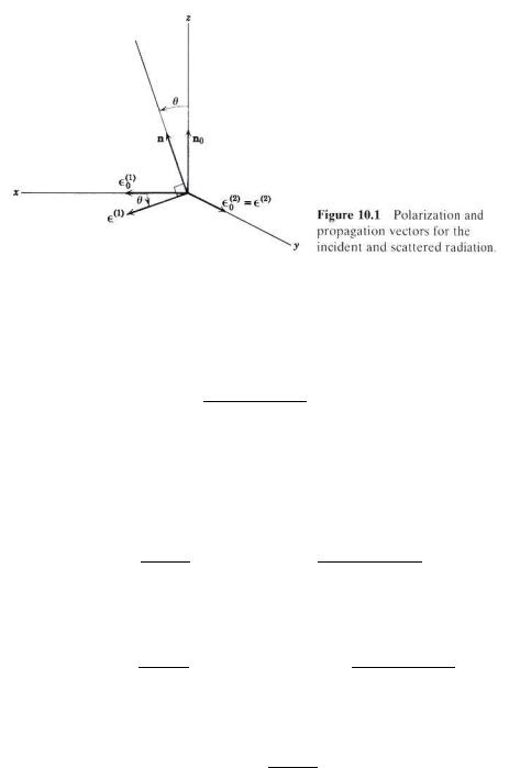
Figure 2: Jackson’s insightful diagram.
and the third orthogonal to the first two,
n − (n · n0)n0
sin θ
In case it is not obvious, the Graham-Schmidt process gave me the third vector. You can check for yourself to see that these vectors are orthogonal and normalized (ˆv ·vˆ = 1). The vector identity given earlier is useful for this. The most general incident scattering wave polarization can be written in terms of these three unit vectors.
!
ǫ = A |
|
n × n0 |
|
+ B (n ) + |
n − (n · n0)n0 |
0 |
sin θ |
0 |
sin θ |
And the most general scattered wave polarization vector can be expressed in terms of the same orthogonal basis.
!
ǫ |
= ǫ |
|
n × n0 |
|
+ ǫ |
(n ) + ǫ |
n − (n · n0)n0 |
|
out |
(1) |
sin θ |
k(1) |
0 |
k(2) |
sin θ |
||
The parallel and perpendicular symbols refer to the polarizations orientation with respect to the scattering plane. We will use the following later:
ˆǫ |
= ǫ |
|
n × n0 |
|
|
(1) |
sin θ |
71

And
!
ǫ |
= ǫ |
(n0) + ǫ |
n − (n · n0)n0 |
|
sin θ |
||||
k |
k(1) |
k(2) |
Proceed by determining the coe cients for the incident wave. We do this be doting the incident wave vector by our basis vectors. Remember that Jackson gives us n0 · ǫˆ0 = 0. We realize immediately that B = 0. The other components are
= ǫˆ0 |
· |
" |
n |
− (sin· |
θ |
0) |
n |
0 |
# = sin θ [n · ǫˆ0 − (n · n0)(n0 · ǫˆ0)] = |
sin θ n · ˆǫ0 |
|||
|
|
|
n |
n |
|
|
|
1 |
|
1 |
|
||
And
A = ǫˆ0 · n × n0 sin θ
Calculate the scattering cross section for an arbitrarily polarized beam is done with the average of the incoming polarization and then the sum of the outgoing polarizations. That means that the total cross section is the sum of the cross sections for the two final polarization states. These states correspond to polarizations perpendicular and parallel to the scattering plane.
dσ |
! |
|
! |
|
|
! |
dΩ |
= |
dΩ k |
+ |
dΩ |
||
T ot |
|
|||||
In order to evaluate the cross sections, it will be helpful to know the following first: ǫk ·ǫ0, ǫ ·ǫ0, n×ǫk, n×ǫ , and n0 ×ǫ0. Rewrite the incident polarization by putting and A in explicitly.
ǫ0 = |
1 |
|
(n · ǫ0)[n − (n0 |
· n)n0] + |
1 |
|
[(n0 × n) · ǫ0](n0 |
× n) |
||||||||||||
|
|
|
|
|||||||||||||||||
sin2 θ |
sin2 θ |
|||||||||||||||||||
Now, take the relevant dot products. |
|
|
|
|
|
|
|
|
|
|
||||||||||
(n |
ˆǫ ) = |
n · ǫˆ0 |
[1 |
− |
(n |
· |
n)2] = |
n · ǫˆ0 |
(1 |
− |
cos2 |
θ) = n |
· |
ǫˆ |
||||||
sin2 θ |
|
|||||||||||||||||||
|
· 0 |
|
|
|
0 |
|
sin2 θ |
|
|
|
0 |
|||||||||
And |
|
|
|
|
|
|
|
|
|
|
|
|
|
|
|
|
|
|
|
|
ǫk · ǫ0 = |
1 |
[−(n · ǫˆ0)(ˆǫ · n0)(n0 · n)] = |
1 |
(n · ǫˆ0)(n0 |
· n) |
|||||||||||||||
|
|
|||||||||||||||||||
sin2 θ |
sin θ |
|||||||||||||||||||
72

And
ǫ |
· ǫ0 = |
1 |
[ˆǫ |
· (n0 × n)][(n0 × n) · ǫˆ0] = |
1 |
[(n0 |
× n) · ˆǫ0] |
|
|
||||||
sin2 θ |
sin θ |
We can also find
ǫk · n0 = − sin θ ǫ · (n0 × n) = sin θ
Now, we have all the dot products needed to find the cross sections.
For the parallel case, the scattering cross section is equation 5 with only ǫˆk in the final polarization.
|
dΩ ! |
= k4a6 |
(ǫk |
· ǫ0)[1 − |
|
2 (n · n0)] + |
2 (n · ǫ0)(ǫk · n0) |
2 |
||||||||||||||||
|
dσ |
|
|
|
|
|
|
|
1 |
|
|
|
|
|
1 |
|
|
|
|
|
|
|||
|
|
|
k |
|
|
|
|
|
1 |
|
|
|
|
|
|
1 |
|
|
|
|
|
2 |
||
|
|
1 |
|
|
|
|
|
|
|
|
|
|
|
(n · ǫˆ0)[− sin θ] |
||||||||||
|
|
|
|
|
|
|
|
|
|
|
|
|
|
|
||||||||||
= k4a6 |
|
|
(n · ǫˆ0)(n0 |
· n)[1 − |
|
|
(n0 |
· n)] + |
|
|
|
|||||||||||||
sin θ |
2 |
|
2 |
|
|
|||||||||||||||||||
|
|
|
|
|
|
= k4a6 |
"(n · ǫˆ0) |
cos θ |
− |
1 |
(cos2 θ + sin2 θ) |
# |
2 |
|||||||||||
|
|
|
|
|
|
|
|
2 |
|
|
|
|
|
|||||||||||
|
|
|
|
|
|
|
|
|
|
|
sin θ |
|
|
|
||||||||||
|
|
|
|
|
|
|
|
|
|
|
|
|
|
4 6 |
"(n · ǫˆ0) |
cos θ − 21 |
|
# |
2 |
|||||
|
|
|
|
|
|
|
|
|
|
|
|
|
= k a |
sin θ |
|
|
||||||||
For the perpendicular case, we do the same as above but instead of ǫˆk, we have ǫˆ in the final polarization.
dΩ ! |
= k4a6 |
|
|
|
|
|
|
|
|
|
|
|
|
|
|
|
|
2 |
|
(ǫ · ǫ0)[1 − 2 (n · n0)] + 2 (n · ǫˆ0)(ˆǫ · n0) |
|||||||||||||||||||
dσ |
|
|
|
|
1 |
|
|
|
1 |
|
|
|
|
|
|
|
|
|
|
|
|
|
|
|
|
|
|
|
1 |
|
(n · n0)] |
2 |
|||||||
|
|
|
|
|
|
|
|
|
|
||||||||||
|
|
|
|
|
|
|
|
|
|
|
|||||||||
|
|
|
|
|
= k4a6 |
(ˆǫ · ˆǫ0)[1 − |
|
|
|
||||||||||
|
|
|
|
2 |
|
||||||||||||||
|
|
|
|
1 |
|
|
|
|
|
|
|
|
|
1 |
|
|
2 |
||
|
|
|
|
|
|
|
|
|
|
|
|
|
|
|
|
||||
|
|
|
= k4a6 |
|
|
[(n0 |
× n) · ǫˆ0] 1 − |
|
|
n0 · n |
|||||||||
|
|
|
sin θ |
2 |
|||||||||||||||
|
|
|
|
4 |
|
6 |
1 |
|
|
|
21 cos θ |
|
2 |
||||||
|
|
|
|
= k a |
"[(n0 × n) · ǫˆ0] |
|
− |
# |
|||||||||||
|
|
|
|
|
sin θ |
||||||||||||||
We add these to get the total cross section.
dσ |
!T ot |
= |
k4a6 |
[n · ǫˆ0]2[cos θ − |
1 |
]2 + [(n0 |
× n) · ˆǫ0]2[1 − |
1 |
cos θ]2 |
|
dΩ |
sin2 θ |
2 |
2 |
73
Multiply out the squares. |
|
|
|
|
|
|
|
|
|
|
|
|
|
|
|
|
|
|
|
|
|
|||||||||||
|
|
|
|
dσ |
|
|
|
k4a6 |
|
|
|
|
|
|
|
|
|
|
|
|
|
|
|
|
5 |
|
|
|||||
|
|
|
|
|
|
! |
= |
|
|
|
|
[n · ǫˆ0]2[(cos2 θ − 1) − cos θ + |
|
|
] |
|
||||||||||||||||
|
|
|
|
dΩ |
sin2 |
θ |
4 |
|
||||||||||||||||||||||||
|
|
|
|
|
|
T ot |
|
|
|
|
|
|
|
|
|
|
|
|
|
|
|
|
|
|
|
|
||||||
|
|
|
|
|
|
k4a6 |
|
|
|
1 |
|
|
|
|
|
|
5 |
− cos θ] |
|
|||||||||||||
|
|
|
|
+ |
|
|
[(n0 × n) · ǫˆ0]2[ |
|
(cos2 θ − 1) + |
|
|
|||||||||||||||||||||
|
|
|
|
sin2 θ |
4 |
4 |
|
|||||||||||||||||||||||||
And then, with some algebra, |
|
|
|
|
|
|
|
|
|
|||||||||||||||||||||||
|
dΩ ! |
= k a |
"−[n · ǫˆ0] |
|
− |
|
4 [(n0 × n) · ˆǫ0 |
] + |
5 |
−cos2 θ |
([n · ˆǫ0 |
] |
||||||||||||||||||||
|
2 |
|
1 |
|||||||||||||||||||||||||||||
|
dσ |
4 6 |
|
|
|
|
|
|
|
1 |
|
|
|
|
|
|
|
2 |
4 |
|
|
cos θ |
|
|
|
2 |
||||||
|
|
T ot |
|
|
|
|
|
|
|
|
|
|
|
|
|
|
|
|
|
|
|
− |
|
|
|
|
||||||
Recall that we were given |
|
|
|
|
|
|
|
|
|
|
|
|
|
|
|
|
|
|
|
|
|
|||||||||||
|
|
|
|
|
|
|
|
|
|
ǫ0 · ǫ0 = 1 → 1 = [ǫ0k]2 + [ǫ0 ]2 |
|
|
|
|
||||||||||||||||||
This means that |
|
|
|
|
|
|
|
|
|
|
|
|
|
|
|
|
|
|
|
|
|
|
|
|
|
|
||||||
|
|
|
|
|
|
|
1 |
|
|
|
|
|
1 |
|
|
|
|
|
|
|
|
|
|
|
|
|||||||
|
|
|
|
|
|
|
|
|
[n · ǫˆ0 |
]2 + |
|
[(n0 |
× n) · ǫˆ0]2 = 1 |
|
|
|
|
|||||||||||||||
|
|
|
|
|
|
|
|
sin2 θ |
sin2 θ |
|
|
|
|
|||||||||||||||||||
Finally, we can report the total cross section. |
|
|
|
|
|
|
|
|
||||||||||||||||||||||||
|
|
|
dΩ ! |
|
= k4a6 |
|
4 |
|
− [ǫ0 · n]2 − 4[n · (n0 × ǫ0)]2 − n0 · n |
|||||||||||||||||||||||
|
|
|
dσ |
|
|
|
|
|
|
5 |
|
1 |
|
|
|
|
|
|
|
|
|
|
||||||||||
|
|
|
|
|
|
T ot |
|
|
|
|
|
|
|
|
|
|
|
|
|
|
|
|
|
|
|
|||||||
Where we replaced cos θ with n0 · n.
#
+ [(n0 × n) · ˆǫ0]2)
(6)
b. If the incident radiation is linearly polarized, show that the
cross section is |
|
|
8(1 + cos2 |
θ) − cos θ − |
8 sin2 |
θ cos 2φ |
|||
|
dΩ ! |
= k4a6 |
|||||||
|
dσ |
|
|
5 |
|
|
3 |
|
|
where n · n0 = cos θ and the azimuthal angle φ is measured from the direction of the linear polarization.
It is a simple matter of geometry to determine the following dot and cross products. I’ll give you a diagram someday, but for now, you’ve got to draw this one yourself.
ǫ0 · n = sin φ sin θ
n · (n0 × ǫ0) = ǫ0 · (n × n0) = ǫ0 · vˆ sin θ = sin θ cos φ
74

Once we have these products, part b is simply a matter of trigonometric formulae and algebraic manipulations. Consider the term in brackets from equation 6, and write the newly revealed angles in.
54 − [ǫ0 · n]2 − 14[n · (n0 × ǫ0)]2 − n0 · n =
54 − sin2 φ sin2 θ − 14 sin2 θ cos2 φ − cos θ
I’m going to fly through this algebra. To start o , I will use cos 2α = 2 cos2 α − 1 = 1 − 2 sin2 α. It should be clear what’s going on.
54 − sin2 φ sin2 θ − 14 sin2 θ cos2 φ − cos θ
=54 − 12(1 − cos 2φ) sin2 θ − 18 sin2 θ(1 − cos 2φ) − cos θ
=58(1 + cos2 θ) − cos θ − 38 sin2 θ cos 2φ
=54 − 12 (1 + cos 2φ) sin2 θ − 18 sin2 θ(1 − cos 2φ) − cos θ = 54 − 58 sin2 θ − 38 sin2 θ cos 2φ − cos θ
=54 − 58(1 − cos2 θ) − 38 sin2 cos 2φ − cos θ
=58 (1 + cos2 θ) − cos θ − 38 sin2 θ cos 2φ
Then, we have what Jackson wants.
dΩ ! |
= k4a6 |
|
8(1 + cos2 |
θ) − cos θ − |
8 sin2 |
θ cos 2φ |
||
dσ |
|
|
5 |
|
|
3 |
|
|
75
Problem 10.11
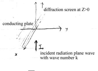
A perfectly conducting flat screen occupies half of the x-y plane (i.e., x < 0 ). A plane wave of intensity I0 and wave number k is incident along the z axis from the region z < 0. discuss the values of the di racted fields in the plane parallel to the x-y plane defined by z = Z > 0. Let the coordinates of the observation point by (X,0,Z).
a. Show that, for the usual scalar Kircho approximation and in
√
the limit Z >> X and kZ >> 1, the di racted field is
|
|
|
|
|
1 + i |
|
eikZ−iωts |
|
2 |
|
∞ eiu2 du |
||||||||
|
|
Ψ = |
I0 |
||||||||||||||||
|
|
2i |
|
π |
|||||||||||||||
|
|
q |
|
|
|
|
|
|
Z−Ξ |
||||||||||
|
1 |
|
|
|
|
|
|
|
|
|
|
|
|
|
|
|
|
|
|
where Ξ = X( |
k |
) 2 . |
|
|
|
|
|
|
|
|
|
|
|
|
|
|
|
|
|
2Z |
|
|
|
|
|
|
|
|
|
|
|
|
|
|
|
|
|
||
|
|
|
|
|
|
k |
|
|
|
|
|
|
|
|
ikrp |
||||
|
|
|
|
|
|
|
|
ZAperture |
e |
|
|
|
|||||||
|
|
Ψ(r0) = |
|
qI0 |
|
dA′ |
|||||||||||||
|
|
2πi |
rp |
|
|||||||||||||||
r0 is the observation point, and rp |
= |
|
(x′ − X)2 |
+ (y′ − Y )2 + (z′ − Z)2 is |
|||||||||||||||
q
the distance from the area point at the aperture to the observation point. The small letters denote the aperture values while the large letters denote values at the observation point. dA′ = dx′dy′ in this case because the screen is in the xy plane.
I proceed first by evaluating the integral over the y coordinate.
∞ eikrp |
|
|
I1 = Z∞ |
|
dy′ |
rp |
||
76