electrodynamics / Companion to J.D. Jackson's Classical Electrodynamics 3rd ed. - R. Magyar

c. Nuclear charge distributions can be approximated by a constant charge density throughout a spheroidal volume of semi-major axis a and semi-minor axis b. Calculate the quadrupole moment of such a nucleus, assuming that the total charge is Zq. Given that Eu153

For the nucleus, the total charge is Zq where q is the charge of the electron. The charge density is the total charge divided by the volume for points inside the nucleus. Outside the nucleus the charge density vanishes. The volume of an general ellipsoid is given by the high school geometry formula, V = 43 πabc. In our case, a is the semi-major axis, and b and c are the semi-minor axes. By cylindrical symmetry b = c.

The nuclear quadrapole moment is defined Q = 1q (3z2 − R2) ρdV . Because

The limits on the second integral are determined because the charge density vanishes outside the limits.

27

28

Problem 4.8

a very long, right circular, cylindrical shell of dielectric constant ǫ

ǫ0

and inner and outer radii a and b respectively, is placed in a previ-

~

ously uniform electric field E0 with the cylinder’s axis perpendicular to the field. The medium inside and outside the cylinder has a dielectric constant of unity. Determine the potential and electric field in the three regions, neglecting end e ects.

Since the total charge is zero, we can use Poisson’s equation:

2Φ = 0

Symmetry in this problem leads me to choose cylindrical coordinates in which the Poisson equation is

Because of translational symmetry along the zaxis, Φ is independent of z, and we need only consider the problem in the r-θ plane.

Try a separation of variables, i.e. Φ(r, θ) = R(r)Θ(θ).

This will give us two equations. The first isn’t too hard to solve.

∂2Θ = −m2 Θ

∂θ2

29

This admits the obvious solution:

Θ(θ) = e±imθ

We’ll employ the convenient linear superposition

Θ(θ) = cos(mθ)

The second equation is a bit trickier.

Let’s guess that

R(r) = r±m, m 6= 0

and

R(r) = ln r + C, m = 0

are solutions. In fact, it is not that hard to show that these are in fact solutions.

The general solution is a linear combination of these solutions. The boundary conditions will determine just what this linear combination is. The uniform external field can be reproduced by Φ = −E0r cos φ. At the surface of the

~

cylinder we have another boundary condition. Namely, at x = a or b, Ek

physical grounds, we can limit the form of the solution outside and inside the cylindrical region. Outside, we need to have the electric field at infinity, but we certainly don’t want the field to diverge. The logarithmic and rn with n > 1 terms diverge as r goes to infinity; clearly, these terms are unphysical.

In between the cylindrical shells, we don’t have any obvious physical constraints.

30

Inside, we have to eliminate the diverging terms at the origin.

∞

Φin = X Dmrm cos(mθ + δm)

m=1

Now, it’s time to match boundary conditions. They were Φ = −E0r cos φ as x → ∞, and at x = a or b; Ek = − and ǫE = −ǫ are continuous. For m 6= 1, we find αm = βm = β−m = δm and Am = Bm = B−m = Dm = 0. We might have suspected that only the m = 0 terms contribute because the only thing that breaks the symmetry in this problem is the external electric field which has m = 1. Note further that for m = 0, A0 = 0, and C = 0. I am left with the following forms:

Outside:

In between the cylinders:

1

Φmid = B−1 r cos(θ + β−1) + B1r cos(θ + β1)

Inside the cylinders:

Φin = D1r cos(θ + δ1)

Because each region has the same symmetry with respect to the external field, we can drop the phases. For the outside region, we find

And inside,

Φin = D1r cos(θ)

31

And

B1a + B−1 = D1a a

b. Sketch the lines of force for a typical case of b 2a.

Since we are only concerned with a qualitative sketch, we’ll consider a particular case. Take κ = 3, E0 = 2 and a2 = 2. Then, we have A1 = −2, B1 = −2, B−1 = −2, and D1 = −1. The potential becomes

2

Φout = −Er cos θ − r cos θ

2 Φmid = −2r cos θ − r cos θ

And

Φin = −r cos θ

Now, I just need to make the plots.

c. Discuss the limiting forms of your solution appropriate for a solid dielectric cylinder in a uniform field, and a cylindrical cavity in a uniform dielectric.

32

For the dielectric cylinder, I shrink the inner radius down to nothing; a → 0.

A1 = κκ −+ 11 b2E0

B1 = −2E0

1 + κ B−1 = 0

−4E0

D1 = (1 + κ)2

For the cylindrical cavity, I place the surface of the outer shell at infinity, b → ∞. In this limit A1 is ill-defined, so we’ll ignore it.

33

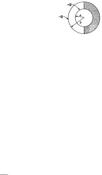
Problem 4.10

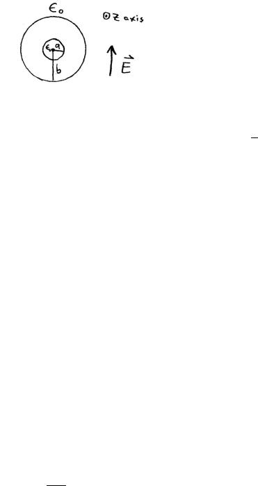
Two concentric conducting spheres of inner and outer radii a and b, respectively, carry charges ±Q. The empty space between the spheres is half-filled by a hemispherical shell of dielectric (of di-

Because of this radial symmetry, we expect that Eθ and Eφ will vanish, and by Gauss’s law, we expect Er to be radially symmetric. Therefore, we need

This has the form of Coulomb’s law but with an e ective total charge, Qef f =

2ǫ0 Q.

ǫ+ǫ0

b. Calculate the surface charge distribution on the inner sphere.

σi = ǫiEr in this case. On the inner surface,

34

c. Calculate the polarization charge density induced on the surface of the dielectric at r = a.

Find the polarization charge density by subtracting the e ective charge density from the total contained charge density: Qef f = Q + Qpol.. This gives

polarization charge over the half the inner sphere’s surface which is in con-

35

Problem 5.1

Starting with the di erential expression

for the magnetic induction at a point P with the coordinate ~x produced by an increment of current Idℓ′ at ~x′, show explicitly that for a closed loop carrying a current I the magnetic induction at P

where Ω is the solid angle subtended by the loop at the point P . This corresponds to a magnetic scalar potential, ΦM = . The sign convention for the solid angle is that Ω is positive if the point P views the “inner” side of the surface spanning the loop, that is, if a unit normal ~n to the surface is defined by the direction of current flow via the right hand rule, Ω is positive if ~n points away from the point P , and negative otherwise.

Biot-Savart’s law tells us how to find the magnetic field at some point P (~r)

~′

produced by a wire element at some other point P2(r ). At P (~r):

There is a form of Stokes’ theorem which is useful here: H dℓ′ × A = R dS′ ×′ × A. I’ll look up a definitive reference for this someday; this maybe on the inside cover of Jackson’s book.

With the useful identity, ′f (x − x′) = f (x′ − x), we have

36