electrodynamics / Companion to J.D. Jackson's Classical Electrodynamics 3rd ed. - R. Magyar

The first term corresponds to the reflection at the n1-n2 interface. The second term is a wave which passes through the n1-n2 interface, reflects o the n2-n3 interface, and then transits through the n1-n2 interface. Higher order terms correspond to multiple internal reflections.

Note the phase change over the internal reflection path. It is 2k2d for one round trip from the n1-n2 to the n2-n3 interface and back. k2 is n2cω . The

~

phase shift makes sense because the term in the exponent is really ik · ~r and

~

the distance is ~r = d for the first leg. On the return leg, the sign of both

~ ~

k and d change because the wave is propagating backwards and over the same distance in the opposite direction as before. The total phase change is the product of these two changes and so ikd + i(−k)(−d) = 2ikd. If you are motivated, you could probably show this with matching boundary conditions. I think this heuristic argument su ces.

I’ll write this series in a suggestive form:

h i h i

r = r12 + t12r23t21e2ik2d × 1 + r23r21e2ik2d + (r23r21)2e4ik2d + ...

The second term in the brackets is a geometric series:

You can obtain for yourself with the help of Jackson page 306:

With these formulae, I’ll show the following useful relationships:

47

1 + 2r12r23 cos(2k2d) + (r12r23)2

R + T = 1 is reasonable if we demand that energy be conserved after a long period has elapsed.

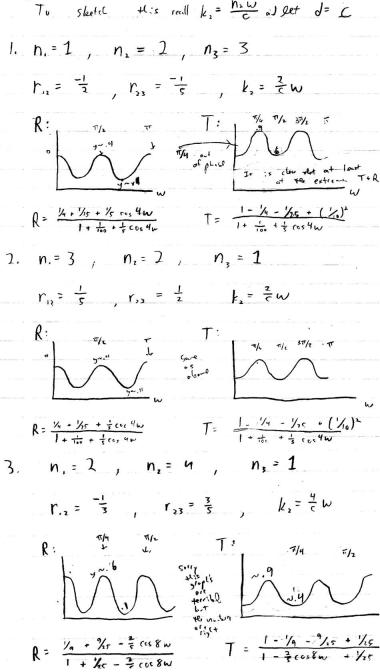
Now, here are all the crazy sketches Jackson wants:

48

Problem 7.12

The time dependence of electrical disturbances in good conductors is governed by the frequency-dependent conductivity (Jackson’s equation 7.58). Consider longitudinal electric fields in a conductor, using Ohm’s law, the continuity equation, and the di erential form of Coulomb’s law.

a. Show that the time-Fourier transformed charge density satisfies the equation:

[σ(ω) − iωǫ0] ρ(ω) = 0

From now on, I’ll drop the subscript f . We both know that I mean free charge and current. From the last equality,

Assume that ρ(t) can be written as the time Fourier transform of ρ(ω). I.e.

ρ(t) = √1 Z ρ(ω)e−iωtdω

2π

Plug ρ(t) into equation 1.

For the integral to vanish the integrand must vanish so

[σ − iωǫ0] ρ(ω)e−iωt = 0

50

For all t. We conclude that

[σ(ω) − iωǫ0] ρ(ω) = 0 b. Using the representation,

σ(ω) = σ0

1 − iωτ

where σ0 = ǫ0ωp2τ and τ is a damping time, show that in the approximation ωpτ >> 1 any initial disturbance will oscillate with the plasma frequency and decay in amplitude with a decay constant λ = 21τ . Note that if you use σ(ω) σ(0) = σ0 in part a, you will

find no oscillations and extremely rapid damping with the (wrong)

decay constant λw = σ0 .

ǫ0

From part a, σ(ω) − iǫ0ω = 0. Let ω = −iα so that

σ(ω) = ǫ0ωp2τ 1 − ατ

And the result from part a becomes σ(ω) − ǫ0α = 0 →

The numerator must vanish. Divide the numerator by τ ǫ0,

α2 − τ −1α + ωp2 = 0

Solve for α.

1 h q i

α = 2 τ −1 ± τ −2 − 4ωp2

If ωp >> 1, we can write α in an approximate form,

α (2τ )−1 ± iωp

The imaginary part corresponds to the oscillations at ωp, the plasma frequency. The real part is the decay in amplitude 21τ .

51

Problem 7.16

Plane waves propagate in an homogeneous, non-permeable, but anisotropic dielectric. The dielectric is characterized by a tensor ǫij , but if coordinate axes are chosen as the principle axes, the components of displacement along these axes are related to the electric field components by Di = ǫiEi, where ǫi are the eigenvalues of the matrix ǫij .

~

a. Show that plane waves with frequency ω and wave vector k must satisfy

52

~

b. Show that for a given wave vector k = k~n there are two distinct

We will write the result in part a as a matrix equation. The non-diagonal

elements of ǫij vanish so we replace ǫij → ǫiiδij . Define a second rank tensor,

↔

T , as

↔

At this point, we can solve det T = 0 for the allowed velocity values.

Or written out explicitly, we have

53

Multiplying out the determinant,

which can be written in a nicer form.

Use n21 + n22 + n33 = 1 to replace the number one in the above equation.

Simplify. In the end, you’ll obtain a relationship for the v values.

54

either vanish or be related in such a way as to preserve the equality. However,

which we have shown to vanish. Therefore, the left hand side is zero, and

~ ~

the right hand side,D1 · D2 = 0. The eigenvectors are perpendicular.

55

Problem 7.22

Use the Kramers-Kr¨onig relation to calculate the real part of ǫ(ω), given the imaginary part of ǫ(ω) for positive ω as . . .

The Kramer-Kr¨onig relation states:

Notice that the real part of ǫ(ω) depends on an integral over the entire frequency range for the imaginary part!

Here, we will use a clever trick.

And this integral is easy to do!

The integral can be evaluated using complex analysis, but I’ll avoid this. The integral is just a Hilbert transformation and you can look it up in a table.

56