reading / DOE docs / 5 DOE-EPRI 2001 cofiring Biomass w. Coal

Some 56 tests were conducted at the Bailly Generating Station, representing over 200 test hours. In total, over 1000 hours were logged on the system firing blends of wood waste and coal, petroleum coke and coal, and triburn blends of wood waste/petroleum coke/coal. The basic analytical tool used for testing was the construction of heat and material balances, complemented by measurement of emissions at the inlet of the air heater. Emissions measured included NOx, CO, and SO2. Stack testing was also performed by Clean Air Engineering, measuring NOx, CO, total hydrocarbons (HC’s), and SO3.

Operationally there were no difficulties with the triburn project. The blends of opportunity fuels did not impact boiler capacity or operability; they did not decrease the temperatures in the cyclone or cause problems with slag tapping. From an efficiency perspective, the blends tended to improve operations since the most favorable blends were 2:1 and 3:1 petroleum coke/urban wood waste. Based upon all of the testing, the following efficiency equation was constructed:

%W is the mass percentage of wood waste in the blend, and %PetC is the mass percentage of petroleum coke in the blend. The r2 value for this equation, with 56 degrees of freedom, is 0.86. The equation itself, and the individual terms in the equation, has significance values ³99.99%; the probability that it occurred randomly was <0.0001. The unburned carbon in the flyash increased with the addition of petroleum coke, and decreased with the addition of wood waste. What became obvious was the fact that the wood waste brought the volatiles to the new fuel, and the petroleum coke provided the heat content.

From an emissions perspective, the triburn project was a success. Figure S-18 depicts the emissions of CO, THC, and SO3 as measured by Clean Air Engineering. Note the very low emissions of all three pollutants.

Figure S-18. Emissions of Carbon Monoxide, Total Hydrocarbons, and Sulfur Trioxide at the Bailly Generating Station Triburn Demonstration (values in ppmvd corrected to 3% O2)

NOx emissions decreased with every opportunity fuel, but particularly with the fuel blends. The equation describing the NOx reduction phenomenon is as follows:

NOx(ppmvd @ 3%O2) = 479 – 6.4(%W), - 6.8(%PetC)+ 0.79(Lm) + 23.0(%O2) [S-11]

NO is expressed in ppmvd at 3% O (dry basis). L is load, or main steam flow, expressed as

x 2 m

tonne/hr of main steam, and %O2 is percent excess O2 on a total basis, recorded by plant instruments at the economizer exit.

Alternatively:

Where NOx is measured in lb/106 Btu, and Le is load, expressed in 103 lb/hr of main steam flow. All other terms are as defined in equation [S-11]. The load term is deceptively low; however the range of steam flows for the unit during the tests was typically 502 tonne/hr (1.1x106 lb/hr of main steam). The r2 for the equations is 0.70. The significance of the %W is 99.999% (the probability that it is a random occurrence is <0.00001) and the significance of the %PetC term is 99.9999% (the probability that it is a random occurrence is <0.000001). The significance of the total equation is about equal to that for the %PetC term. The fuel blend, with the fuels reported on an individual basis, and the load and excess O2 terms can be used to explain 70% of the NOx emissions. Included in the 30% unexplained impacts on NOx emissions are the synergies between the wood waste and the petroleum coke, as shown in Figure S-19. Note that the equation generated from the triburn test line shows that the minimum NOx

formation will be generated at 40 percent cofiring of the designed opportunity fuel blend. The combination of the two fuels exceeds the additive value of the two fuels taken individually.

The Bailly program also documented that the triburn program could be used to reduce mercury, lead, and other metal emissions. The Bailly triburn test program, then, provided significant additional information regarding the process of cofiring.

Figure S-19. NOx Emissions Measured During the Bailly Triburn Tests

CONCLUSIONS FROM THE TEST PROGRAM OF THE COOPERATIVE AGREEMENT

The testing and demonstration sponsored by EPRI, and then supported by the EPRI-USDOE Cooperative Agreement, documented the following:

∙Cofiring can be used as a cost-effective means for reducing greenhouse gas emissions, providing utilities with a low capital cost option

∙Cofiring can be accomplished in a manner that does not negatively impact the operability or operations of a given power plant, provided that the most appropriate cofiring technology is applied

∙Cofiring virtually always reduces the power plant boiler efficiency, however the reductions can be managed as an economic issue rather than as a technical barrier

∙Cofiring can be used to reduce virtually all airborne emissions, and has a particularly beneficial impact on NOx emissions.

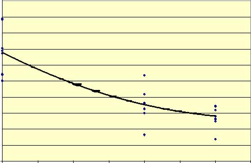
With respect to the NOx emissions, the evidence of impacts is substantial. Figure S-20 depicts the NOx emissions from all tests sponsored by the EPRI-USDOE Cooperative Agreement. Note the line indicating where a 1 percent cofiring percentage (heat input basis) would equal a 1 percent NOx reduction. This line represents the substitution effect of a low nitrogen fuel. Note that over 67 percent of all tests are well above that line. Figure S-20 shows considerable spread in the data. This spread is caused by variations in firing technology, biomass fuel used, percentage of biomass fuel used, base coal fired, and combustion conditions (e.g., load, excess O2). Despite this variability, however, the impact of cofiring on NOx emissions is highly significant.

Average NOx Emissions Reduction

Percent Cofiring, Btu Basis

Figure S-20. NOx Reduction Caused by Cofiring—All Tests Sponsored by the EPRI-USDOE Cooperative Agreement

SPECIAL STUDIES ASSOCIATED WITH THE EPRI-USDOE COOPERATIVE AGREEMENT

In addition to the cofiring tests and demonstrations, the EPRI-USDOE Cooperative Agreement was used to support significant engineering studies used to expand the potential of cofiring. These studies included:

∙An assessment of gasification-based cofiring at the Allen Fossil Plant, evaluating the ability of gasification to address issues of flyash contamination from biomass, the ability of gasification to further promote NOx reduction, and the ability of gasification to broaden the base of appropriate biomass resources (Foster Wheeler Development Corporation, 1998). The fuel supply data developed during this study included not only sawdust but also non-recyclable paper, clean urban wood waste, bark, cotton gin trash, and other locally available materials. The study considered integrating biomass gasification with the use of wastewater treatment gas to be supplied to the plant. This was followed by a Request for Proposals by TVA to construct and test gasificationbased cofiring. The project was not pursued beyond the RFP stage.

∙The development of detailed fuels databases, including some rudimentary modeling of cofiring combustion (see Prinzing, 1996). This database development included information on biomass and various types of coal, sufficient for initial analyses of cofiring.

∙The development of a survey of all cofiring testing by utilities—including those that did not participate in the EPRI-USDOE Cooperative Agreement (see Battista, 2001). A previous study (Wiltsee, 1998) included cofiring in a broader survey of biomass technologies.

FUTURE RESEARCH REQUIREMENTS TO COMMERCIALIZE COFIRING

The current status of cofiring has been well documented (see Plasynski, Goldberg, and Chen, 2001; Tillman, 2000; Tillman, Plasynski, and Hughes, 1999; Tillman, Hughes, and Plasynski, 1999; Freeman, Goldberg, and Plasynski, 1998). The EPRI-USDOE Cooperative Agreement has moved the technology towards full commercial deployment. Certain issues remain that must be addressed by additional demonstrations, testing, or research. These include:

∙Broadening the useful biomass fuel base either by technologies to make more difficult residues more useful (e.g., gasification, fluidized bed combustion) or by pre-treatment technologies

∙Addressing the issues associated with biomass ash including the potential for catalyst deactivation in selective catalytic reduction (SCR) systems, the problems associated with marketing flyash, and related considerations

∙Integrating biomass cofiring into gas-fired technologies, particularly combined cyclecombustion turbine generation, as a means to ensure long-term viability of this fuel source

∙Developing a deeper understanding of the properties of biomass fuels—including crops proposed as fuels—to ensure compatibility with coal and to ensure the ability to maximize the benefits from these biofuels

∙Developing and demonstrating technologies that have special applications for biomass (e.g., the use of biomass or producer gas from biomass as a reburn fuel)

While the Cooperative Agreement has served a highly useful purpose of advancing cofiring to the point of initial commercialization, additional research can profitably be employed to broaden the application of this technology. And, given the role of electricity in the US energy arena, broadening the application of cofiring may be the best near-term approach to increasing the contribution and role of biomass as a renewable energy resource.

1.0.INTRODUCTION

1.1.THE BASIS FOR FOCUSING ON COFIRING

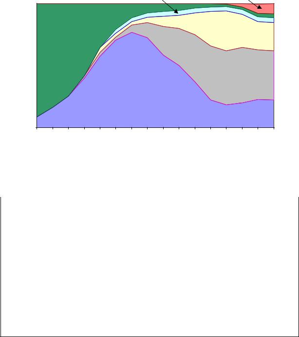
Increasing the use of renewable fuels in the US economy—both in absolute and relative contributions— has long been a goal of energy planners and policy makers in both the public and private sectors. Achieving such increases requires recognizing long term trends shown in Figures 1-1 and 1-2, indicating that the US economy increasingly has focused upon energy dense fossil fuels to meet the economy’s need for low cost, abundant energy supplies. It also recognizes the need to continue the trends shown in Table 1-1, documenting the fact that biomass fuels have consistently increased their contribution to the US economy since 1970, both in absolute and relative terms.

The goal or objective of increasing the use of renewable fuels in the US economy also requires recognition of trends within the distribution of energy use in the US. The dominant trend is increased electrification, as shown in Figure 1-3. Energy use for electricity generation has grown dramatically— particularly as a percentage of total energy use. On an absolute basis, fuel use for non-electricity and non-transportation applications has remained somewhat static and, in many sectors, has declined. In 1970 the US consumed 51.9x1015 Btu/yr for non-electricity uses and 16.4x1015 Btu for electricity generation. In the year 2000, energy consumption for non-electricity purposes grew to 61.3x1015 Btu/yr, with most of the growth coming in the transportation sector. Energy consumption for electricity generation in the year 2000 was 35.1x1015 Btu/yr. Biomass, which now supports some 7,000 MWe of electricity generating capacity, has grown slowly in this marketplace. In 1960 and 1970, some 0.3x1015 Btu/yr of wood, agricultural materials, and municipal refuse was used to generate electricity. In 1980 that number had increased to 0.4x1015 Btu, in 1990 it was 0.6x1015 Btu, and at the turn of the century it had increased to 0.7x1015 Btu. Much of that biomass was fired in cogeneration applications within the pulp and paper industry, although small stand-alone wood-fired power plants have been built in Vermont, Washington, Maine, California, Virginia, and other locations.

Electricity generation, then, provides a highly useful target market for increasing the use of renewable energy resources within the US. Further, electricity generating stations firing, or cofiring biomass can be dispatched to meet demand; dispatchability makes biomass a useful energy source for utilities. Biomass cofiring in existing power plants is one of two general pathways for increasing the use of this family of fuels in the electricity sector. The other pathway is the construction of stand-alone biomass-fired power plants. Trends in the construction of generating stations favor cofiring. Individual steam boiler-steam turbine combinations have increased in capacity over time, as shown in Figure 1-4. By 1996, the average new boiler ordered was 650 MWe (UDI, 2000). Typically boilers constructed since 1980 are either 2400 psig/1000oF/1000oF drum boilers or 3500 psig/1000oF/1000oF supercritical boilers. These are very large installations. Comparable trends are being experienced in the combustion turbinecombined cycle (CCCT) arena, where new installations >500 MWe are now common as well. Biomass installations >70 MWe are not practical due to logistical and fuel supply issues; at such low capacities it is virtually impossible to justify, economically, the efficiency enhancements associated with reheat cycles.

Reheat is virtually always installed on new steam power plants, and is being designed into heat recovery steam generators (HRSG’s) for CCCT installations as well.

Energy Consumption in the US

Figure 1-1. Historical Trends in US Energy Consumption by Fuel

(Sources: Energy Information Agency; 2000; Enzer, Dupree, and Miller, 1975)

EnergyConsumptionPercentagebyFuel

Figure 1-2. Historical Trends in Percentage Distribution of US Energy Consumption (Sources: Energy Information Agency, 2000; Enzer, Dupree, and Miller, 1975)

Table 1-1. Biomass Contribution to US Energy Production and Consumption

Sources: Energy Information Agency 2000; Energy Information Agency, 2001; Norwood and Warnick, 1982; Schreuder and Tillman, 1980; Tillman, 1977; Tillman, 1978; Enzer, Dupree, and Miller, 1975

Fuel Consumption by Use

Figure 1-3. Importance of Electricity Generation in US Fuel Consumption (Source: Energy Information Agency, 2000)

Average MW per Boiler

TimePeriod

Figure 1-4. Average Capacity of Steam-Electric Generating Systems Installed, 1940 – 1995. (Source: Utility Data Institute, 1996)