

2174 |
CHAPTER 27. CONTROL VALVES |
The common pneumatic signal approach (one controller, one I/P transducer) is simple but su ers from the disadvantage of slow response, since one I/P transducer must drive two pneumatic actuators. Response time may be improved by adding a pneumatic volume booster between the I/P and the valve actuators, or by adding a positioner to at least one of the valves. Either of these solutions works by the same principle: reducing the air volume demand on the one common I/P transducer.
Wiring two I/P transducers in series so they share a common signal current is another way to split-range two control valves. This approach does not su er from slow response, since each valve has its own dedicated I/P transducer to supply it with actuating air. We now have a choice where we implement the split ranges: we can do it in the I/P transducers (i.e. each I/P transducer having a di erent calibration) or in the control valves (i.e. selecting control valve actuators having di erent factory bench-set pressure ranges). The convenience of re-ranging I/P transducers compared to purchasing new valve actuators with custom bench-set ranges, and the superior response time of dedicated transducers over a common I/P, makes the dual-transducer approach more popular.
A disadvantage of the series-wired I/P strategy is the extra burden placed on the controller’s output signal circuitry: one must be careful to ensure the two series-connected I/P converters do not drop too much voltage at full current, or else the controller may have di culty driving both devices in series. Another (potential) disadvantage of series-connected valve devices in one current loop is the inability to install “smart” instruments communicating with the HART protocol, since multiple devices on the same loop will experience address conflicts24. HART devices can only work in hybrid analog/digital mode when there is one device per 4-20 mA circuit.
A popular way to implement split-ranging is to use multiple 4-20 mA outputs on the same controller. This is very easy to do if the controller is part of a large system (e.g. a DCS or a PLC) with multiple analog output channels. If multiple outputs are configured on one controller, each valve will have its own dedicated wire pair for control. This tends to result in simpler wiring than series-wired I/P transducers or positioners, since each valve loop is a standard 4-20 mA circuit just like any other (non-split-ranged) control valve loop circuit. It may also be the most practical way to implement split-ranging when “smart” valve positioners are used, since the dedicated loop circuits allow for normal operation of the HART protocol with no address conflicts.
An advantage of dual controller outputs is the ability to perform the split-range sequencing within the controller itself, which is often easier than re-ranging an I/P or calibrating a valve positioner. This way, the 4-20 mA signals going to each valve will be unique for any given controller output value. If sequenced as such, the I/P transducer calibration and valve bench-set values may be standard rather than customized. Of course, just because the controller is capable of performing the necessary sequencing doesn’t mean the sequencing must be done within the controller. It is possible to program the controller’s dual analog outputs to send the exact same current signal to each valve, configuring each valve (or each positioner, or each I/P transducer) to respond di erently to the identical current signals.
24Although the HART standard does support “multidrop” mode where multiple devices exist on the same current loop, this mode is digital-only with no analog signal support. Not only do many host systems not support HART multidrop mode, but the relatively slow data communication rate of HART makes this choice unwise for most process control applications. If analog control of multiple HART valve positioner devices from the same 4-20 mA signal is desired, the address conflict problem may be resolved through the use of one or more isolator devices, allowing all devices to share the same analog current signal but isolating each other from HART signals.

27.11. SPLIT-RANGING |
2175 |
A digital adaptation of the dual-output controller sequencing method is seen in FOUNDATION Fieldbus systems25, where a special software function block called “SPLT” exists to provide splitranged sequencing to two valves. The “SPLT” function block takes in a single control signal and outputs two signals, one output signal for each valve in a split-ranged pair. The function block diagram for such a system appears here:
|
|
|
|
|
|
|
|
|
|
|
|
|
|
|
|
|
|
|
|
BKCAL |
_IN |
|
|
|
BKCAL_OUT CAS_IN |
|
|
|
BKCAL_OUT |
|
Valve A |
|
|
|
|||||
|
|
|
|
|
|
|
|
|
|
||||||||||
|
|
|
|
|
|
|
|
|
|
|
|
|
|
|
|
|
|
|
|
CAS_IN |
|
|
|
|
BKCAL_IN_1 |
|
SPLT |
|
OUT_1 CAS_IN |
|
|
|
BKCAL_OUT |
||||||
|
|
|
|
|
|
|
|
|
|||||||||||
|
|
|
|
|
|
|
|
|
|||||||||||
|
|
|
|
|
|
|
|
|
|
|
|
|
|
|
|
|
|
|
|
FF_VAL |
|
|
|
OUT |
BKCAL_IN_2 |
|
|
OUT_2 |
|
|
|
|
|
|
|||||
|
|
|
|
|
|
|
AO |
OUT |
|
||||||||||
|
|
|
|
|
|
|
|
|
|
|
|
|
|
|
|
||||
|
IN |
|
PID |
|
|
|
|
|
|
|
|
|
|||||||
|
|
|
|
|
|
|
|
|
|
|
|
|
|
|
|
|
|||
|
|
|
|
|
|
|
|
|
|
|
|
|
|
||||||
TRK_IN_D |
|
|
|
|
|
|
|
|
|
|
|
|
|
|
|
|
|
|
|
|
|
|
|
|
|
|
|
|
|
|
|
|
|
|
|
|
|
||
|
|
|
|
|
|
|
|
|
|
|
|
|
|
|
|
|
|
||
TRK_VAL |
|
|
|
|
|
|
|
|
|
|
|
CAS_IN |
|
Valve B |
BKCAL_OUT |
||||
|
|
|
|
|
|
|
|
|
|
|
|
||||||||
|
|
|
|
|
|
|
|
|
|
|
|
|
|
||||||
|
|
|
|
|
|
|
|
|
|
|
|
|
|
|
|
||||
|
|
|
|
|
|
|
|
|
|
|
|
|
|
|
|||||
|
|
|
|
|
|
|
|
|
|
|
|
|
|
|
|
|
|
|
|
|
|
|
|
|
|
|
|
|
|
|
|
|
|
|
AO |
OUT |
|
|
|
|
|
|
|
|
|
|
|
|
|
|
|
|
|
|
|
|
|
|
|
|
|
|
|
|
|
|
|
|
|
|
|
|
|
|
|
|
|
|
|
|
|
|
|
|
|
|
|
|
|
|
|
|
|
|
|
|
|
|
|
|
|
|
|
|
|
|
|
|
|
|
|
|
|
|
|
|
|
|
|
In this Fieldbus system, a single PID control block outputs a signal to the SPLT block, which is programmed to drive two unique positioning signals to the two valves’ AO (analog output) blocks. It should be noted that while each AO block is unique to its own control valve, the SPLT and even PID blocks may be located in any capable device within the Fieldbus network. With FOUNDATION Fieldbus, control system functions are not necessarily relegated to separate devices. It is possible, for example, to have a control valve equipped with a Fieldbus positioner actually perform its own PID control calculations and split-ranged sequencing by locating those function blocks in that one physical device!
Dual controllers are an option only for specialized applications requiring di erent degrees of responsiveness for each valve, usually for exclusive or progressive split-ranging applications only. Care must be taken to ensure the controllers’ output signals do not wander outside of their intended ranges, or that the controllers do not begin to “fight” each other in trying to control the same process variable26.
25To review, Fieldbus is an all-digital industrial control protocol, where instruments connect to a control system and to each other by means of a single network cable. Signals are routed not by specific wire connections, but rather by software entities called function blocks whereby the engineer or technician programs the instruments and control system what to do with those signals. The function blocks shown in this example would typically be accessed through the graphic display of a DCS in a real Fieldbus system, lines drawn between the blocks instructing the system where each of the instrument signals need to go.
26Both controllers should be equipped with provisions for reset windup control (or have no integral action at all), such that the output signal values are predictable enough that they behave as a synchronized pair rather than as two separate controllers.
2176 |
CHAPTER 27. CONTROL VALVES |
An important consideration – and one that is easily overlooked – in split-range valve systems is fail-safe mode. As discussed in a previous section of this chapter (on section 27.7.3), the basis of fail-safe control system design is that the control valve(s) must be chosen to fail in the mode that is safest for the process in the event of actuating power loss or control signal loss. The actions of all other instruments in the loop should then be selected to complement the valves’ natural operating mode.
In control systems where valves are split-ranged in either complementary or exclusive fashion, one control valve will be fully closed and the other will be fully open at each extreme end of the signal range (e.g. at 4 mA and at 20 mA). If the sequencing for a set of complementary or exclusive splitranged control valves happens after the controller (e.g. di erent actuator actions) the valves must fail in opposite modes upon loss of controller signal. However, if it is deemed safer for the process to have the two valves fail in the same state – for example, to both fail closed in the event of air pressure or signal loss – we may use dual sequenced controller outputs, achieving either complementary or exclusive control action by driving the two valves with two di erent output signals. In other words, split-ranging two control valves so they normally behave in opposite fashion does not necessarily mean the two valves must fail in opposite states. The secret to achieving proper failure mode and proper split-range sequencing is to carefully locate where the sequencing takes place in the control system.
27.11. SPLIT-RANGING |
2177 |
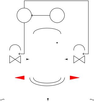
As an example of a split-ranged system with opposite valve failure modes, consider the following temperature control system supplying either hot water or chilled water to a “jacket” surrounding a chemical reactor vessel. The purpose of this system is to either add or remove heat from the reactor as needed to control the temperature of its contents. Chemical piping in and out of the reactor vessel has been omitted from this P&ID for simplicity, so we can focus just on the reactor’s temperature control system:
Output "b" 0% = 4 mA
100% = 20 mA
|
|
|
|
|
|
TIC |
|
TT |
|
|
|
|
|
||||||||
|
|
|
|
|
|
37 |
|
|
37 |
|
|
|
|
|
|
|
|
||||
|
Output "a" |
|
|
|
|
|
|
|
|
|
|
|
|
|
|
|
|
||||
|
|
|
|
|
|
|
|
|
|
|
|
|
|
|
|
||||||
|
0% = 4 mA |
|
|
|
|
|
|
|
|
|
|
|
|
|
|
|
|
||||
|
100% = 20 mA |
|
|
|
|
|
|
|
|
|
|
|
|||||||||
TV-37a |
|
|
|
|
|
TV-37b |
|||||||||||||||
|
|
|
|
|
|||||||||||||||||
|
|
|
|
|
|
|
|
|
|
|
Reactor |
|
|
|
|
|
|
|
|
||
|
|
|
|
|
|
|
|
|
|
|
|
|
|
|
|
|
|
|
|||
|
|
|
|
|
|
|
|
|
|
|
|
|
|
|
|
|
|
|
|
|
|
|
|
|
|
|
|
|
|
|
|
|
|
|
|
|
|
|
|
|
|
||
|
|
|
P |
|
|
|
|
|
|
|
|
|
|
|
|
|
P |
|
|
||
|
|
|
|
|
|
|
|
|
|
|
|
|
|
|
|
|
|
|
|
|
|
|
|
FC |
|
|
|
|
|
|
|
|
|
|
|
FO |
|||||||
|
4 mA = fully closed |
|
|
|
|
|
|
4 mA = fully open |
|||||||||||||
12 mA = fullly closed |
|
|
|
|
|
|
12 mA = fullly closed |
||||||||||||||
|
20 mA = fully open |
|
|
|
|
|
|
20 mA = fully closed |
|||||||||||||
|
|
|
|
|
|
|
|
|
|
|
|
|
|
|
|
|
|
|
|
|
|
|
|
|
|
|
|
|
|
|
|
|
|
|
|
|
|
|
|
|
|
|
|
|
|
|
|
|
|
|
|
|
|
|
|
|
|
||||||||
4 mA |
20 mA |
|
|
|
|
4 mA |
|
|
20 mA |
||||||||||||
|
|
|
|
|
|
|
|
|
|
|
|
|
|
|
|
|
|
|
|
|
|
|
|
|
|
|
|
|
|
|
|
|
|
|
|
|
|
|
|
|
|
|
|
From hot |
Return to |
From cold |
water supply |
heating/cooling |
water supply |
|
systems |
|
Here, the controller has been configured for dual-output operation, where the output value drives two identical 4-20 mA signals to the control valve positioners, which directly input the current signals from the controller without the need for I/P transducers in between. The hot water valve (TV-37a) is fail-closed (FC) while the cold water valve (TV-37b) is fail-open (FO). Half-range positioner calibrations provide the exclusive sequencing necessary to ensure the two valves are never open simultaneously – TV-37b operates on the lower half of the 4-20 mA signal range (4-12 mA), while TV-37a operates on the upper half (12-20 mA).
Consider the e ects from the controller (TIC-37) losing power. Both 4-20 mA signals will go dead, driving both valves to their fail-safe modes: hot water valve TV-37a will fully close, while cold water valve TV-37b will fully open. Now consider the e ects of air pressure loss to both valves. With no air pressure to operate, the actuators will likewise spring-return to their fail-safe modes: once again hot water valve TV-37a will fully close, while cold water valve TV-37b will fully open. In both failure events, the two control valves assume consistent states, ensuring maximum cooling to the reactor in the event of an output signal or instrument air failure.
2178 |
CHAPTER 27. CONTROL VALVES |
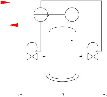
However, suppose we desired both of these valves fail in the closed position in the event of an output signal or instrument air failure, rather than have the cooling valve fail open while the heating valve fails closed. Clearly this would require both TV-37a and TV-37b to be fail-closed (FC), which would mean we must find some other way to sequence their operation to achieve split ranging. Examine this reconfiguration of the reactor temperature control system, using identical control valves (signal-to-open, fail-closed) for both hot and cold water supply, and a controller with exclusively-sequenced 4-20 mA output signals:
|
|
|
|
Output "b" |
|
|
|
|
0% = 20 mA |
|
|
|
|
50% = 4 mA |
|
|
|
||
0% |
100% 100% = 4 mA |
|||
TIC |
TT |
37 |
37 |
|
|
|
|
Output "a" |
|
|
|
|
0% = 4 mA |
|
|
|
|
|
0% |
100% |
50% = 4 mA |
||
|
||||
100% = 20 mA
TV-37a |
|
|
|
TV-37b |
|||||||||
|
|
|
|
|
|
Reactor |
|
|
|
|
|
|
|
|
|
|
|
|
|
|
|
|
|
|
|
||
|
|
|
|
|
|
|
|
|
|
|
|
|
|
|
|
|
|
|
|
|
|
|
|
|
|
||
|
|
P |
|
|
|
|
|
|
|
P |
|
||
|
|
|
|
|
|
|
|
|
|
|
|
|
|
|
FC |
|
|
|
|
|
FC |
||||||
4 mA = fully closed |
|
|
|
|
4 mA = fully closed |
||||||||
20 mA = fully open |
|
|
|
|
20 mA = fully open |
||||||||
|
|
|
|
|
|
|
|
|
|
|
|
|
|
|
|
|
|
|
|
|
|
|
|
|
|
|
|
|
|
|
|
|
|
|
|
|
|
|
|
|
|
From hot |
Return to |
From cold |
water supply |
heating/cooling |
water supply |
|
systems |
|
Consider the e ects from the controller (TIC-37) losing power. Both 4-20 mA signals will go dead, driving both valves to their fail-safe modes: fully closed. Now consider the e ects of air pressure loss to both valves. With no air pressure to operate, the actuators will spring-return to their fail-safe modes: once again both control valves fully close. In both failure events, the two control valves consistently close. The failure modes of both valves are still consistent regardless of the nature of the fault, but note how this scheme allows both valves to fail in the same mode if that is what we deem safest for the process.
As with all fail-safe system designs, we begin by choosing the proper fail-safe mode for each control valve as determined by the safety requirements of the process, not by what we would consider the simplest or easiest-to-understand instrument configurations. Only after we have chosen each valve’s failure mode do we choose the other instruments’ configurations. This includes split-range sequencing: where and how we sequence the valves is a decision to be made only after the valves’ fail-safe states are chosen based on process safety.
27.12. CONTROL VALVE SIZING |
2179 |
27.12Control valve sizing
When control valves operate between fully open and fully shut, they serve much the same purpose in process systems as resistors do in electric circuits: to dissipate energy. Like resistors, the form that this dissipated energy takes is mostly heat, although some of the dissipated energy manifests in the form of vibration and noise27.
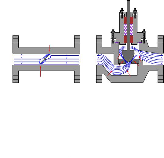
In most control valves, the dominant mechanism of energy dissipation comes as a result of turbulence introduced to the fluid as it travels through constrictive portions of the valve trim. The following illustration shows these constrictive points within two di erent control valve types (shown by arrows):
Globe valve
Butterfly valve
Note: red arrows show points of maximum fluid energy loss
The act of choosing an appropriate control valve for the expected energy dissipation is called valve sizing.
27Valve noise may be severe in some cases, especially in certain gas flow applications. An important performance metric for control valves is noise production expressed in decibels (dB).
2180 |
CHAPTER 27. CONTROL VALVES |
27.12.1Physics of energy dissipation in a turbulent fluid stream
Control valves are rated in their ability to throttle fluid flow much in the same way resistors are rated in their ability to throttle the flow of electrons in a circuit. For resistors, the unit of measurement for electron flow restriction is the ohm: 1 ohm of resistance results in a voltage drop of 1 volt across that resistance given a current through the resistance equal to 1 ampere:
V
I 


 I
I
R
Arrows point in direction of conventional flow
The mathematical relationship between current, voltage, and resistance for any resistor is Ohm’s Law :
R =
V
I
Where,
R = Electrical resistance in ohms
V = Electrical voltage drop in volts
I = Electrical current in amperes
Ohm’s Law is a simple, linear relationship, expressing the “friction” encountered by electric charge carriers as they slowly drift through a solid object.
When a fluid moves turbulently through any restriction, energy is inevitably dissipated in that turbulence. The amount of energy dissipated is proportional to the kinetic energy of the turbulent motion, which is proportional to the square of velocity according to the classic kinetic energy equation for moving objects:
Ek = 12 mv2
If we were to re-write this equation to express the amount of kinetic energy represented by a volume of moving fluid with velocity v, it would look like this:
Kinetic energy per unit volume = 12 ρv2
We know that the amount of energy dissipated by turbulence in such a fluid stream will be some proportion (k) of the total kinetic energy, so:
Energy dissipated per unit volume = 12 kρv2
27.12. CONTROL VALVE SIZING |
2181 |
Any energy lost in turbulence eventually manifests as a loss in fluid pressure downstream of that turbulence. Thus, a control valve throttling a fluid flowstream will have a greater upstream pressure than downstream pressure (assuming all other factors such as pipe size and height above ground level being the same downstream as upstream):
P = P1 - P2
P1 
 P2
P2
Q 

 Q
Q
R
This pressure drop (P1 − P2, or P ) is equivalent to the voltage drop seen across any currentcarrying resistor, and may be substituted for dissipated energy per unit volume in the previous equation28. We may also substitute QA for velocity v because we know volumetric flow rate (Q) is the product of fluid velocity and pipe cross-section area (Q = Av) for incompressible fluids such as liquids:
P1 − P2 |
= 2 kρ |
A |
|
2 |
|||
|
|
1 |
|
Q |
|
||
|
|
|
|
|
|
|
|
Next, we will solve for a quotient with pressure drop (P1 − P2) in the numerator and flow rate (Q) in the denominator so the equation bears a resemblance to Ohm’s Law (R = VI ):
1 Q2
P1 − P2 = 2 kρ A2
P1 − P2 = kρ
Q2 2A2
√r
P1 − P2 |
= |
|
kρ |
|
Q |
2A2 |
|||
|
||||
28In case you were wondering, it is appropriate to express energy loss per unit volume in the same units of measurement as pressure. For a more detailed discussion of dimensional analysis, see section 2.11.13 beginning on page 208 where Bernoulli’s equation is examined and you will see how the units of 12 ρv2 and P are actually the same.

2182 |
CHAPTER 27. CONTROL VALVES |
Either side of the last equation represents a sort of “Ohm’s Law” for turbulent liquid restrictions: the left-hand side expressing fluid “resistance” in the state variables of pressure drop and volumetric flow, and the right-hand term expressing fluid “resistance” as a function of fluid density and restriction geometry. We can see how pressure drop (P1 − P2) and volumetric flow rate (Q) are not linearly related as voltage and current are for resistors, but that nevertheless we still have a quantity that acts like a “resistance” term:
|
√ |
|
R = |
P1 − P2 |
|
|
|
Q |
Where,
R = Fluid “resistance”
P1 = Upstream fluid pressure P2 = Downstream fluid pressure Q = Volumetric fluid flow rate
k = Turbulent energy dissipation factor ρ = Mass density of fluid
A = Cross-sectional area of restriction
r
R =
kρ
2A2
The fluid “resistance” of a restriction depends on several variables: the proportion of kinetic energy lost due to turbulence (k), the density of the fluid (ρ), and the cross-sectional area of the restriction (A). In a control valve throttling a liquid flow stream, only the first and last variables are subject to change with stem position, fluid density remaining relatively constant.
In a wide-open control valve, especially valves o ering a nearly unrestricted path for moving fluid (e.g. ball valves, eccentric disk valves), the value of A will be at a maximum value essentially equal to the pipe’s area, and k will be nearly zero29. In a fully shut control valve, A is zero, creating a condition of infinite “resistance” to fluid flow.
It is customary in control valve engineering to express the “restrictiveness” of any valve in terms of how much flow it will pass given a certain pressure drop and fluid specific gravity (Gf ). This measure of valve performance is called flow capacity or flow coe cient, symbolized as Cv . A greater flow capacity value represents a less restrictive (less “resistive”) valve, able to pass greater rates of flow for the same pressure drop. This is analogous to expressing an electrical resistor’s rating in terms of conductance (G) rather than resistance (R): how many amperes of current it will pass with 1 volt of potential drop (I = GV instead of I = VR ).
If we return to one of our earlier equations expressing pressure drop in terms of flow rate, restriction area, dissipation factor, and density, we will be able to manipulate it into a form expressing flow rate (Q) in terms of pressure drop and density, collecting k and A into a third term which will become flow capacity (Cv ):
1 Q2
P1 − P2 = 2 kρ A2
29In a case of minimal throttling, almost none of the fluid’s kinetic energy is lost to turbulence, but rather passes right through the valve unrestricted.
27.12. CONTROL VALVE SIZING |
2183 |
First, we must substitute specific gravity (Gf ) for mass density (ρ) using the following definition of specific gravity:
|
|
Gf = |
|
|
|
ρ |
|
|
|
|
|
|
|
|
|
|
|||||||||
|
|
|
|
|
|
|
|
|
|
|
|
|
|
|
|
|
|||||||||
ρwater |
|
|
|
|
|
|
|
|
|
|
|||||||||||||||
|
|
ρwater Gf = ρ |
|
|
|
|
|
|
|
|
|
|
|||||||||||||
Substituting and continuing with the algebraic manipulation: |
|
||||||||||||||||||||||||
|
|
|
|
|
|
1 |
|
|
|
|
|
|
|
|
|
|
Q2 |
|
|||||||
P1 − P2 = |
|
kρwater Gf |
|
|
|
|
|
|
|
|
|||||||||||||||
2 |
A2 |
|
|||||||||||||||||||||||
|
|
P1 − P2 |
= |
|
1 |
kρwater |
Q2 |
|
|
|
|
|
|||||||||||||
Gf |
2 |
A2 |
|
||||||||||||||||||||||
|
|
|
|
|
|
|
|
|
|
|
|||||||||||||||
|
|
2A2 |
|
|
|
P1 − P2 |
|
= Q2 |
|
||||||||||||||||
kρwater |
|
|
|
|
|
||||||||||||||||||||
|
|
|
Gf |
|
|
|
|
|
|
|
|
|
|||||||||||||
Q = |
|
2A2 |
|
P1 − P2 |
|
|
|||||||||||||||||||
|
|
s |
|
|
s |
|
|
|
|
|
|
|
|||||||||||||
|
|
kρwater |
|
Gf |
|
||||||||||||||||||||
|
|
|
|
|
|
|
|
|
|
|
|
|
|
|
|
|
|
|
|||||||
|
|
|
|
|
|
|
|
|
|
|
|
|
q |
|
2A2 |
|
|||||||||
The first square-rooted term in the equation, |
|
, is the valve capacity or Cv |
factor. |
||||||||||||||||||||||
kρwater |
|||||||||||||||||||||||||
Substituting Cv for this term results in the simplest form of valve sizing equation (for incompressible fluids):
s
Q = Cv
P1 − P2
Gf
In the United States of America, Cv is defined as the number of gallons per minute of water that will flow through a valve with 1 PSI of pressure drop30. A similar valve capacity expression used with metric units rates valves in terms of how many cubic meters per hour of water will flow through a valve with a pressure drop of 1 bar. This latter flow capacity is symbolized as Kv .
For the best results predicting required Cv values for control valves in any service, it is recommended that you use valve sizing software provided by control valve manufacturers. The formulae shown here do not account for all factors31 influencing fluid flow rate and pressure drop, and therefore yield approximate values only. Modern valve sizing software is easy to use, especially when referenced to specific models of control valve sold by that manufacturer, and is able to account for a diverse multitude of factors a ecting proper sizing.
30The specification of certain British units of measurement for flow and pressure drop means that there is more to
2A2 |
|
|
Cv than just q kρwater |
. Cv |
also incorporates a factor necessary to account for the arbitrary choice of units. |
31Such factors include fluid compressibility, viscosity, specific heat, vapor pressure to name a few. Not only will modern valve sizing software more accurately predict valve sizes for particular applications than these simple formulae, but this software may also provide estimations of noise levels produced by the valve.
2184 |
CHAPTER 27. CONTROL VALVES |
Control valve sizing is complex enough that some valve manufacturers used to give away “slide rule” calculator devices so customers could choose the Cv values they needed with relative ease. Photographs of a two-sided valve sizing slide rule are shown here for historical reference: