Proceedings of 6th International Conference of Young Scientisis on Solutions of Applied Problems in Control and Communications

forces and its inertia tensor, which determines its response to rotational torques. Body coordinate systems define local coordinate systems, one of them is CG – body’s center of gravity another are C S, they are associated with joints to the body block.

Constraints were translated into revolute blocks. Revolute block represents one rotational degree of freedom. The follower body rotates relative to the base body about a single rotational axis going through collocated body coordinate system origins. Sensor and actuator ports can be added. In model were twelve revolute blocks which represented 12 degrees of freedom (DoF).

Edit SimMechanics model

At first I reduced DoFs from twelve to six by changing revolute blocks which were connected to cylinders for weld blocks. Weld block represents joint between base and follower with zero degrees of freedom. To this block is possible to add a sensor but not an actuator. Afterwards I run a simulation. As shown in the Fig. 4, individual parts of model were collided between themselves during the simulation.

Fig. 4. Simulation

First step to avoid collisions and also to solve main task which is to get arm at the desired location is adding sensor and actuator to every revolute block of model. Joint actuator actuates a joint block connected between two bodies with one of these signals:

− generalized force (force for translational motion along a prismatic joint primitive / torque for rotational motion about a revolute joint primitive),

91

−motion (translational motion for a prismatic joint primitive, in terms of linear position, velocity, and acceleration / rotational motion for a revolute joint primitive, in terms of angular position, velocity, and acceleration).

The import is the Simulink input signal. The output is the connector port which can be connect to the joint block in case of to want to actuate. A joint actuator block actuates one joint primitive at a time:

−primitive joint (prismatic or revolute) has only one primitive within the joint to actuate;

−composite joint has multiple joint primitives within and i tis neccessery to choose which of those primitives to actuate with the joint actuator.

Joint sensor measures linear or angular position, velocity, acceleration, computed force or torque and reaction force or torque of a joint primitive. Outputs are Simulink signals. Multiple output signals can be bundled into one signal.

To every sensor I connected scope block which displays input signals with respects to the simulation time. To every actuator I joined one sine wave, two derivatives, but to actuator can be connected only one signal, so I these three signals connected to mux (Fig. 5). Mux is used for combine many inputs into single output. Way of connection is at figure.

Sine wave block outputs a sinusoidal waveform. The block can operate in time-based or sample-based mode. In time-based mode is output of the sine wave determined by:

y=amplitude×sin( frequency× time+phase)+bias.

Time specify whether to use simulation time as the source of values for the time variable or an external source. If is specified an external time source, the block displays an input port for the time source. Amplitude defines the amplitude of the signal, default is 1. Bias points out the constant value added to the sine to produce the output of this block. Frequency is in radians per second, default is 1. This parameter appears only in condition of setting Sine type to time-based. Phase specify the phase shift in radians. The default is 0. This parameter appears only in case of setting Sine type to time-based.

Derivative block approximates the derivative of the input signal u with respect to the simulation time t. Is possible to obtain the approximation of

du/dt

92

by computing a numerical difference ∆u/∆t, where ∆u is the change in input value and ∆t is the change in time since the previous simulation (major) time step. This block accepts one input and generates one output. The initial output for the block is zero.

Fig. 5. Connection

Before testing this connection I clicked at Joint Actuator and changed „Actuate with“ from generalized forces to motion. T hen I ran a simulation with default values from Sine Wave (amplitude, frequency = 1, bias, phase, sample time = 0). According to parameters formula of Sine Wave was changed into:

y=amplitude×sin( frequency× time).

In next step I clicked at scope and it showed behaviour of Revolute1 (Fig. 6). From figure is possible to deduce that amplitude of Revolute1 moves in range <1;-> and time in which amplitude reach for first time value (-1) is 1.6 s. From that I calculated frequence by formula

x = 1.6 / 10 (simulation time)

After that I changed value of frequency at 0.16 (rad/sec) and again I run simulation and observed scope (Fig. 7). I did this procedure with every revolute block in model.

93

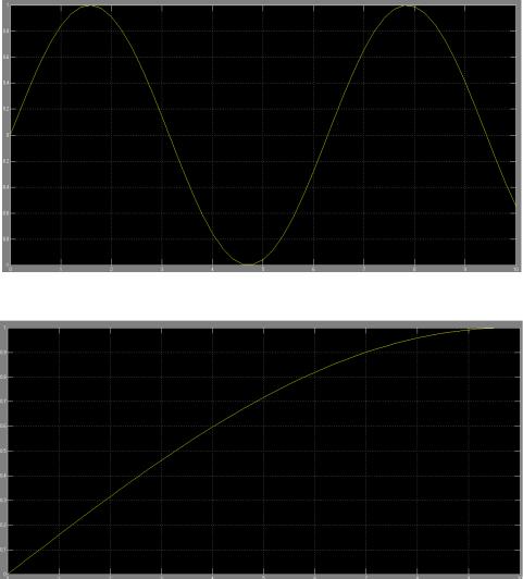
Fig. 6. Scope1

Fig. 7. Scope2

In the Fig. 7 can be seen that amplitude is in range <0;1> so part of arm gets into desired value during simulation time and arm does not cross value bigger than value which is entered from sine wave block. According to this information is SimMechanics model ready to be controlled from Graphical User Interface.

Create GUI

Before creating GUI I had to find out values of amplitudes, in which individual parts collided between themselves and also I recalculated values of

94

amplitudes into values of angles, for example revolute2 amplitude = 51,5 is the same as angle between base and part joined to the base. Value of this angle is 0 degrees.

Then I developed an algorithm, that according to coordinates in carthesian coordinates system calculate amplitudes in sine wave in every revolute block. First step was to deter minate length of arm (Fig. 8).

Fig. 8. Mea surments

Base, P1, and P2 are measurements from CAD model, but P3 is measurement, which is changing according to width of gripped object (Fig. 9). Width of object(a), coordinates (x, y, z) are entered from GUI, base, P1, P2, r and b are defined at the beginnin g of code in GUI.

Fig. 9. G ripper

In Object is P3 calculated accordin g to the formula:

&3 = Br6 − L (M8N )6O

6 .

95

In Object2 is P3 calculated accordinng to the formula:

&3 = Br6 − L (N8M )6O

6 .

P3 is basically a distance from grip per to the object.

For calculating angles I created an algorithm, which is shown in the Fig. 10.

Fig. 10. Algo rithm A

In first step the algorythm calcu late „f“ according to Phytagoras

afterwords it calculate angle „ α“ withα = siusningY goniometric function:

Z,

this angle represents amplitude in Revolute1.

Procedure of calculating of angles „ β“ and „ γ“ is explained in the Fig . 11.

Fig. 11. Algo rithm B

96

If y > base

β= β1 + β2 else

if β1 > β2

β= β1 – β2

else if β1< β2

„ γ“ represents Revolute3, „ β“ represen ts Revolute5. Next step is computes angles in the gripper (Fig. 12).

Fig. 12. Al gorithm C

97

Angle „ ε“ is calculated according a formula:

ε = sin )f,

if is „a“ bigger than „b“ it is computed by:

ε = (cos f) W 90

) .

„ ε“ represents both revolute blocks involved into gri pping (Revolute5,Revolute6). In next step it recalculates angles into amplitudes and it passes data into SimMechanics model. To check if are amplitudes correct, serve function „Check in 3D plot“. This function dr aws lines according to dimensions of arm and according to coordinates entered from GUI. It helps to check if is the position of arm in SimMechanics that, as it should be.

Conclusion

To demonstrate functionality of this work serves three figure. In the Figure 13 is design of GUI with coordinates and with calculated amplitudes, in the Figure 14 is position arm in SimMechanics, and in the Figure 15 is 3D check plot.

Fig. 13. GUI

98

Fig. 14. Arm

Fig. 15. 3D plot

As can bee seen at Fig. 14, marked part has dimension 80 mm from the bottom of the base, so position of arm is a few mm above that mark. At Figure 15 is position of arm at similar value. From that is can be deduce, that arm is possible to get at desired location and is also possible to set gripper which fits to the wide of object.

99

АВТОМАТИЗАЦИЯ РОБОТИЗИРОВАННОЙ РУКИ

Томаш Станович

Словацкий технический университет, факультет материаловедения и техники, г. Трнава, Словакия

Аннотация. Эта статья содержит информацию о проектировании 3D CAD-модели в Autodesk Inventor, его переносе и контроле в MatLab SimMechanics. Первая часть содержит инструкции, как спроектирована роботизированная рука. В частности, каким образом можно создать отдельные части и их дальнейший монтаж. Вторая часть описывает способ перевода CAD-модели в SimMechanics. Следующая часть об обработке модели и о подключении блоков Simulink к блокам SimMechanics. Последняя часть описывает разработку алгоритма расчета амплитуд от координат. Эта часть также включает в себя информацию о создании графического пользовательского интерфейса (GUI) для передачи на рассчитанные амплитуды в SimMehcanics.

Ключевые слова: CAD-модель, SimMechanics, графический интерфейс, амплитуды, алгоритм.

100