


C H A P T E R 6
Density dependence
Introduction
The parameters considered up to this point in this book have been descriptive parameters of a single population. As such, they are most appropriately estimated by properly designed and statistically soundly based surveys or observations of the population in question. This will not always be possible, but is at least an ideal to be targeted. From here on, however, the parameters involve interactions, either between individuals in a single population, the topic of this chapter, or between individuals of different species. Interaction parameters often cannot be measured easily by simple observation of the interacting entities. The ideal way of measuring an interaction is with a manipulative experiment, in which one or more of the interacting entities is perturbed, and the response of the other entities measured. Unfortunately, ecological experiments in natural conditions, at appropriate scale, with controls, and with sufficient replication are very difficult and expensive to undertake, and in some cases are quite impossible. This and the following chapters therefore contain a number of ad hoc approaches that lack statistical rigour, but, provided they are interpreted with due caution, may permit at least some progress to be made with model building.
Importance of density dependence
There has been a long and acrimonious debate amongst ecologists concerning the importance of density-dependent processes in natural populations (e.g. Hassell et al., 1989; Hanski et al., 1993b; Holyoak & Lawton, 1993; Wolda & Dennis, 1993). This book is not the place to review that controversy. All modellers are convinced of the importance of density dependence, for the simple reason that population size in any model will tend rapidly to either extinction or infinity unless the parameters of the model are carefully adjusted so that net mortality exactly balances net fecundity. It seems implausible that this could happen in nature unless some factor (density dependence) acts to perform the adjustment in real populations. This is not to say, however, that density dependence must act on all populations all of the time, nor that real populations spend most of their time at some ‘carrying capacity’ set by densitydependent factors. What is necessary is that, at some times and at some population level, the population should decline because it is at high density. A good
157
158 C H A P T E R 6
working definition of density dependence is provided by Murdoch and Walde (1989): ‘Density dependence is a dependence of per capita growth rate on present and/or past population densities’.
Why do you need an estimate of density dependence?
There are two reasons why you might want to estimate one or more parameters to quantify density dependence. First, you might be trying to fit a model to a time series of population size or density. Such models may perhaps be used to draw indirect inferences about some of the mechanisms affecting population size, but the primary objective of the model-building process is either to describe the time series statistically or to be able to project the population size into the future, together with some idea about the possible range of future values. Such a projection, based only on the properties of the time series to date, will only be valid if the same processes that have determined the time series until the present continue to operate in essentially the same way into the future. The general principles that apply to the fitting of any statistical model should apply in this case: additional terms should only be included in the model if they improve the fit according to a significance level specified in advance. For the purposes of prediction, as distinct from hypothesis testing, one may be able to justify a significance level above the conventional p = 0.05. Nevertheless, in a purely statistical fitting exercise, the logical necessity for density dependence to exist at some density is not, in itself, a justification for including it in the model.
The second major reason for estimating density dependence is to include it in a mechanistic model. As discussed above, some density dependence is essential in many models to keep the results within finite bounds. To omit it because a time series or set of experiments failed to detect it will cause the model to fail.
The easiest way of including generic density dependence in a continuoustime model is via a simple logistic relationship:
dN |
|
|
N |
|
|
|
= rN 1 |
− |
|
. |
(6.1) |
dt |
|
||||
|
|
K |
|
||
Here, r is the intrinsic rate of growth, and K is the carrying capacity. The form
dN |
= rN − kN 2 |
(6.2) |
|
||
dt |
|
|
is identical mathematically; here k (= r/K ) is a parameter describing the strength of the density dependence. Usually, there will be additional terms tacked on to the right-hand side to represent other factors (harvesting, predation, etc.) being modelled.
The same thing can be done in a discrete-time model, but a possible

D E N S I T Y D E P E N D E N C E 159
Table 6.1 Forms for expressing density dependence in discrete time. Density-dependent survival can be represented in the following general form: S = Nf (N ), where S is the number of survivors, N is the number of individuals present initially, and f (N ) is the proportional survival as a function of the initial density. This table, modified from Bellows (1981), displays some forms that have been suggested for this function. The first three forms are single-parameter models, which inevitably are less flexible at representing data than are the final four two-parameter models. Bellows fitted the two-parameter models to two sorts of insect data: experimental studies which recorded numbers of survivors as a function of numbers present initially (set 1, 16 data sets) and long-term census data (set 2, 14 data sets, some field, some laboratory). The final two columns show the number of times each model fitted the data sets best, using nonlinear least squares
|
f (N ) |
k value (log(N/S) ) |
Set 1 |
Set 2 |
|
|
|
|
|
1 |
N −b |
bln N |
|
|
2 |
exp(−aN ) |
aN |
|
|
3 |
(1 + aN )−1 |
ln(1 + aN ) |
|
|
4 |
exp(−aN b) |
aNb |
2 |
3 |
5 |
(1 + (aN)b)−1 |
ln(1 + (aN)b) |
10 |
9 |
6 |
(1 + aN )−b |
bln(1 + aN ) |
1 |
0 |
7 |
(1 + exp(bN − a))−1 |
ln(1 + exp(bN − a)) |
3 |
2 |
problem is that high values of k may cause population size to become negative. Bellows (1981) provides an excellent review of the various functional forms with which density dependence can be represented in discrete time, particularly in insect populations (see Table 6.1).
It is worth emphasizing that logistic density dependence is a very stylized way of including density dependence in a model. Few real populations have been shown to follow such a growth curve. In fact, most basic textbooks use the same example of logistic growth in the field: that of sheep in Tasmania (Odum, 1971; Krebs, 1985; Begon et al., 1990). That this highly unnatural population is used as the standard example of ‘natural’ logistic population growth is a good indication of the rarity of this mode of population growth. Nevertheless, the simplicity and generality of this model make it an appropriate way to represent density dependence when detail is either unavailable or unnecessary. The simple linear form the logistic assumes for density dependence can also be considered as the first term in a Taylor series expansion of a more general function representing density dependence. (A Taylor series is a representation of a function by a series of polynomial terms.)
Quick and dirty methods for dealing with density dependence in models
Omission to obtain conservative extinction risks
In some cases, it may be appropriate to omit density dependence from a mechanistic model, despite the logical necessity for its existence. An example

160 C H A P T E R 6
is the use of stochastic models for population viability analysis (Ginzburg et al., 1990). The problem in population viability analysis is to predict the risk of ‘quasi-extinction’, which is the probability that a population falls beneath some threshold over a specified time horizon. As populations for which this is an important question are always fairly rare, estimating all parameters, but especially those concerned with density dependence, is very difficult. The effect of direct density dependence, if it is not extreme, is to act to bring a population towards an equilibrium. Ginzburg et al. (1990) suggest that a model omitting density dependence will therefore produce estimates of quasi-extinction risks that are higher than they would be in the presence of density dependence. This will lead to conservative management actions.
To use this idea in practice, it is necessary to adjust the estimates of survival and fecundity used in the model so that the rate of increase r is exactly 0. This is effectively assuming that the initial population size is close to the carrying capacity, so that the long-run birth and death rates are equal. If the initial r is less than 0, extinction would be certain, although density dependence might ‘rescue’ the population through lower death rates or higher birth rates once the population had declined. Conversely, if the initial r is greater than 0, the extinction rate will be underestimated by omitting density dependence, because the population may become infinitely large.
This approach is potentially useful over a moderate time horizon. In the very long run, the random walk characteristics of a population model with r = 0 would cause it to depart more and more from the trajectory of a population that was even weakly regulated around a level close to the initial population size of the random walk.
There are substantial difficulties of estimating survival and fecundity in the wild (see Chapter 4). If a clear population trend is not evident, quasi-extinction probability predictions made by adjusting r to equal 0 are likely to be superior to those obtained by using the best point estimates of survival and fecundity in most cases, given the sensitivity of population trajectories to these parameters.
Scaling the problem away
In many deterministic models, the variable defining population size can be considered to be density per unit area. The unit of area is essentially arbitrary, and population size can therefore be rescaled in any unit that is convenient. Defining it in units of carrying capacity eliminates the need to estimate a separate parameter for density dependence. In many cases, such a scaling is helpful in interpreting the results of the model anyway. For example, if a model is developed to investigate the ability of a parasite or pathogen to depress a host population below its disease-free level (see, for example, Anderson, 1979; 1980; McCallum, 1994; McCallum and Dobson 1995), then it makes good sense to define the disease-free population size as unity.

D E N S I T Y D E P E N D E N C E 161
This approach is much less likely to be useful in a stochastic model, because the actual population size, rather than some scaled version of it, is of central importance in determining the influence of stochasticity, particularly demographic stochasticity.
Estimating the ‘carrying capacity’ for a population
The problem of quantifying density dependence in a simple model with logistic density dependence is one of determining a plausible value for the carrying capacity of the population, as set by all factors other than those included explicitly in the formulation of the model. A little thought and examination of eqn (6.1) will show that the carrying capacity is not the maximum possible size of the population. It is rather the population density above which the unidentified density-dependent factors will, on average, cause the population to decline. This population level is unlikely to be identifiable easily, except in special cases. For example, suppose a model is being constructed of a harvested population. Assuming that the population was at some sort of steady state, the average population density before harvesting commenced would be a natural estimate of the carrying capacity. Unfortunately, for many exploited populations, the data needed to calculate a long-term mean density before the commencement of harvesting are unavailable.
In many cases, factors in the model other than the unspecified density dependence will be acting on the population, and the mean population density will not estimate K. Frequently ad hoc estimates, based on approximate estimates of peak numbers, have been used (e.g. Hanski and Korpimäki, 1995). For the reasons discussed in the previous paragraph, this method should be one of last resort.
Statistically rigorous ways of analysing density dependence
One of the primary reasons why the debate over density dependence persists is that it is remarkably difficult, for a variety of technical reasons, to detect density dependence in natural, unmanipulated ecological systems. As detecting the existence of density dependence is statistically equivalent to rejecting a null hypothesis that some parameter describing density dependence is equal to zero, it is correspondingly difficult to quantify the amount of density dependence operating in any real population.
Analysis of time series
Many approaches have been suggested for detecting density dependence in ecological time series. Most of these have been criticized on statistical grounds.
Recent developments in the theory of nonlinear time-series analysis

162 C H A P T E R 6
(see, for example, Tong, 1990) show considerable promise for quantifying and detecting density dependence. Although it is unlikely that there will ever be a single ‘best test’ for density dependence, we now seem to be at a point where reliable, statistically valid methods for examining density dependence in ecological time series have been established. For a recent review, see Turchin (1995).
Dennis and Taper (1994) propose the following model, described as a ‘stochastic logistic’ model:
Nt+1 = Nt exp(a + bNt + σ Zt). |
(6.3) |
Here, Nt is the population size, or some index derived from it, at time t, a and b are fitted constants, and σ Zt is a ‘random shock’ or environmental perturbation, with a normal distribution and variance σ 2. The model is thus a generalization of the Ricker model (see Box 2.1), with random variation added.
Before discussing the technical details of parameterizing this model, it is worth noting a few of its features that may limit its application. First, the variation is ‘environmental stochasticity’. This is not a model that deals explicitly with the demographic stochasticity that may be important in very small populations. Second, the population size next year depends only on that in the current year, together with random, uncorrelated noise. This means that the model does not allow for the possibility of delayed effects, such as may occur if the density dependence acts through a slowly recovering resource or through parasitism or predation (see Chapters 9 and 10; or Turchin, 1990). Finally, the model assumes that all the variation is ‘process error’. That is, the available data are records of the actual population size or index, with no substantial observation error. Handling both types of error simultaneously is difficult, but is possible, provided the observation error can be independently characterized (see Chapter 11).
Nevertheless, provided appropriate statistical checks are made (see below) the model is sufficiently simple to be a workable predictive model for population dynamics including density dependence.
The first step in analysis is to define Xt = ln Nt and Yt = Xt+1 − Xt. Then eqn (6.3) becomes:
Yt = a + b exp Xt + σ Zt. |
(6.4) |
This looks as if it should be amenable to solution by a linear regression of Yt versus Xt. Both can easily be calculated from a time-series population size Nt, and the ‘random shock’ term σ Zt looks essentially the same as the error term in a regression. Up to a point, ordinary linear regression can be used.
There are three possible models of increasing complexity. The simplest model is a random walk, with no density dependence and no trend. Thus, a = 0 and b = 0. The only quantity to be estimated is the variance σ 2. Next, there is

D E N S I T Y D E P E N D E N C E 163
Table 6.2 Parameter estimates for the model of Dennis and Taper (1994)
Model |
* |
( |
|
|
|
|
|
|
F2 |
|
|
|
|
|
|
|
|
|
|
|
|
|
|
|
|
|
|
|
|
|
|
|
|
|
|
|
|
Random walk |
0 |
0 |
|
|
|
|
|
|
|
|
|
1 |
q |
|
|
|
|
|
|
|
|
|
|
|
|
|
|
F |
2 |
= |
∑ y2 |
|
|
|
|
|
|
|
|
|
|
|
|
|
|
|
|
|
|
|
|
|
||||
|
|
|
|
|
|
|
|
|
|
0 |
|
|
t |
|
|
|
|
|
|
*1 = [ |
|
|
|
|
|
|
|
|
|
|
q t =1 |
|
|
|
|
|
|
Exponential growth |
0 |
|
|
|
|
|
|
|
|
|
1 |
q |
|
|
|
|
|
|
|
|
|
|
|
|
|
|
|
F |
2 |
= |
∑(y |
− [)2 |
|
|
|||
|
|
|
|
|
|
|
|
|
|
|
|
|||||||
|
|
|
|
|
|
|
|
|
|
1 |
|
|
t |
|
|
|
|
|
|
|
|
|
|
|
|
|
|
|
|
|
q t =1 |
|
|
|
|
|
|
Logistic |
*2 = [ − (2) |
|
|
|
q |
|
|
|
|
|
|
1 |
q |
|
|
|
|
|
|
|
|
∑(y |
− [)(n |
− )) |
F |
2 |
= |
∑(y |
− * |
|
− ( |
|
n )2 |
||||
|
|
|
|
|
2 |
2 |
||||||||||||
|
|
|
|
|
|
|||||||||||||
|
|
( |
|
= |
t |
|
t −1 |
|
|
2 |
|
|
t |
|
|
t −1 |
||
|
|
2 |
t =1 |
|
|
|
|
|
|
q t =1 |
|
|
|
|
|
|||
|
|
|
|
q |
|
|
|
|
|
|
|
|
|
|
|
|
|
|
|
|
|
|
|
∑(n |
− ))2 |
|
|
|
|
|
|
|
|
|
|
||
|
|
|
|
|
|
t −1 |
|
|
|
|
|
|
|
|
|
|
|
|
t =1
Here, nt is the population size at time t; yt = xt − xt−1, and q is the number of transitions in the time series.
the possibility of exponential growth, with no density dependence (b = 0). Finally, there is the full model with all three parameters to be estimated. Formulae for the estimators are given in Table 6.2.
The estimators are simply as one would expect from elementary regression methods using least squares. If there is no trend or density dependence, the variance of the Yt is simply the average of the squared values. If there is trend, the best estimate of the rate of increase is the mean of Yt, and its variance is as generated from the usual formula. In both these cases, the standard errors, etc. given by any regression package will be perfectly valid.
In the full model, both a and b must be estimated, but the formulae are still simply those one would get from a conventional least squares regression with Nt−1 as the predictor and Yt as the response. The estimated variance F 22 is also simply the mean square error from a regression. The problem is that the full model violates the assumptions of conventional regression, because of its autoregressive structure (Xt appears on both sides of eqn (6.4)). This means that the usual hypothesis-testing methods and ways of calculating standard errors are not valid.
Dennis and Taper (1994) suggest bootstrapping the estimates (see Chapter 2). In this particular case, the method involves a parametric bootstrap. The parameters a, b and σ 2 are estimated by the formulae above and then used to repeatedly generate artificial time series of the same length as the observed series, using eqn (6.4). From each artificial series, new bootstrapped estimates of the parameters can be generated. When a frequency distribution of these is produced, a 95% bootstrapped confidence interval is then just the range between the 2.5th and 97.5th percentiles. Box 6.1 shows an application of this approach to long-term census data for a population of birds.
164 C H A P T E R 6
Box 6.1 Density dependence in silvereyes from Heron Island, Great Barrier Reef
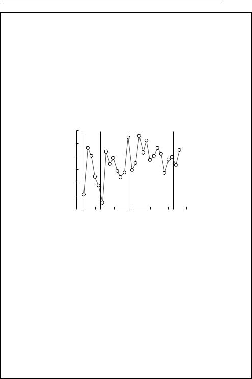
Silvereyes (Zosterops lateralis) are a small terrestrial bird common in eastern Australia and on many south Pacific islands. The population on Heron Island, Great Barrier Reef, has been studied for over 30 years by Jiro Kikkawa (University of Queensland). As the island is very small, the population essentially closed, and almost all individuals are banded, the population size used below can be considered to be a complete census, not an estimate.
The following graph, from Kikkawa, McCallum and Catterall (in preparation), shows the time series of the observed data from the period 1965 –95, with cyclones marked as dashed lines:
|
500 |
|
|
|
|
|
|
|
450 |
|
|
|
|
|
|
Population |
400 |
|
|
|
|
|
|
350 |
|
|
|
|
|
|
|
300 |
|
|
|
|
|
|
|
|
|
|
|
|
|
|
|
|
250 |
|
|
|
|
|
|
|
200 |
|
|
|
|
|
|
|
1965 |
1970 |
1975 |
1980 |
1985 |
1990 |
1995 |
|
|
|
|
Year |
|
|
|
Following Dennis and Taper (1994), the following model was fitted to the data:
Nt+1 = Nt exp(a + bNt + σ Zt)
where Nt+1 is the population size at time t + 1, Nt is the population size at time t, a is a drift or trend parameter, b is a density-dependent parameter, and Zt is random shock to the growth rate, assumed to have a normal distribution with a standard deviation σ.
Note that the above equation can be written as
|
|
N |
|
|
|
|
ln |
|
t+1 |
|
= a + bN |
+ σZ |
, |
|
||||||
|
Nt |
t |
t |
|
||
|
|
|
|
|
|
meaning that the rate of increase between one year and the next is a linear function of the population size. The transformed data are shown below with declines associated with cyclones shown as solid points:
continued on p. 165

D E N S I T Y D E P E N D E N C E 165
Box 6.1 contd
|
1.0 |
|
|
|
|
|
|
)r( |
|
|
|
|
|
|
|
increaseof rate |
0.5 |
|
|
|
|
|
|
0.0 |
|
|
|
|
|
|
|
Finite |
|
|
|
|
|
|
|
|
|
|
|
|
|
|
|
|
–0.5 |
|
|
|
|
|
|
|
200 |
250 |
300 |
350 |
400 |
450 |
500 |
Population size
Least squares (and also maximum likelihood) estimates of these parameters can be calculated using a standard linear regression of Yt+1 = ln(Nt+1/Nt) versus Nt and are given below.
|
Estimate |
Standard error |
t Stat |
p-value |
Lower 95% |
Upper 95% |
||||
|
|
|
|
|
|
|
|
|
|
|
a |
0.730 |
9 |
0.216 |
4 |
3.37 |
0.002 5 |
0.284 |
3 |
1.177 |
5 |
b |
− 0.003 |
12 |
0.000 |
932 |
−3.35 |
0.002 7 |
− 0.005 |
05 |
− 0.001 |
2 |
σ0.204 8
However, the usual standard errors are not valid because of the autoregressive structure of the model. Instead, 2000 time series of the same length as the observed series, and with the same starting point, were generated, and the three parameters estimated from each, generating a parametric bootstrap distribution. The bootstrapped estimates are shown below:
|
Estimate |
Standard error |
Lower 95% |
Upper 95% |
||||
|
|
|
|
|
|
|
|
|
a |
0.970 |
6 |
0.175 |
2 |
0.640 |
07 |
1.315 |
8 |
b |
−0.002 |
50 |
0.000 |
454 |
−0.003 |
400 |
−0.001 |
674 |
σ |
0.176 |
2 |
0.025 |
40 |
0.128 |
6 |
0.226 |
70 |
|
|
|
|
|
|
|
|
|
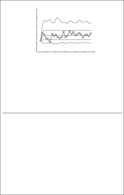
Hence, there is clear evidence of density dependence in the time series, as the bootstrapped confidence interval for b does not include 0.
The mean population trajectory, with 90% confidence bounds (dashed) and maxima and minima of simulated series (dotted), is shown below, together with the actual trajectory (open squares).
continued on p. 166
Box 6.1 contd
|
1000 |
|
|
|
|
|
|
|
800 |
|
|
|
|
|
|
Population |
600 |
|
|
|
|
|
|
400 |
|
|
|
|
|
|
|
|
|
|
|
|
|
|
|
|
200 |
|
|
|
|
|
|
|
0 |
|
|
|
|
|
|
|
1965 |
1970 |
1975 |
1980 |
1985 |
1990 |
1995 |
|
|
|
|
Year |
|
|
|
The time series thus shows very clear evidence of density dependence, around an equilibrium population size of about 380. There are two main caveats, however. First, the noise in this system is clearly not normal. Cyclones are the major perturbation, and these occur discretely in certain years. Second, inspection of the time series suggests that there may be some qualitative change in it occurring after about 1981. The population declined steadily after the two previous cyclones, but did not do so after the 1979 cyclone.
Density dependence in fledging success
The following table shows the number of individuals attempting to breed, the numbers banded as nestlings and their percentage survival from 1979 to 1992:
|
No. attempting |
No. banded |
% surviving until |
No. surviving until |
Year |
to breed |
at nest |
1st breeding |
1st breeding |
|
|
|
|
|
1979 |
383 |
301 |
13.95 |
42 |
1980 |
314 |
287 |
13.94 |
40 |
1981 |
327 |
324 |
27.47 |
89 |
1982 |
370 |
259 |
22.39 |
58 |
1983 |
368 |
319 |
19.75 |
63 |
1984 |
348 |
281 |
16.73 |
47 |
1985 |
328 |
282 |
17.38 |
49 |
1986 |
317 |
231 |
31.17 |
72 |
1987 |
316 |
139 |
22.3 |
31 |
1988 |
365 |
301 |
15.28 |
46 |
1989 |
288 |
392 |
23.47 |
92 |
1990 |
317 |
369 |
20.87 |
77 |
1991 |
335 |
309 |
22.01 |
68 |
1992 |
315 |
237 |
20.68 |
49 |
|
|
|
|
|
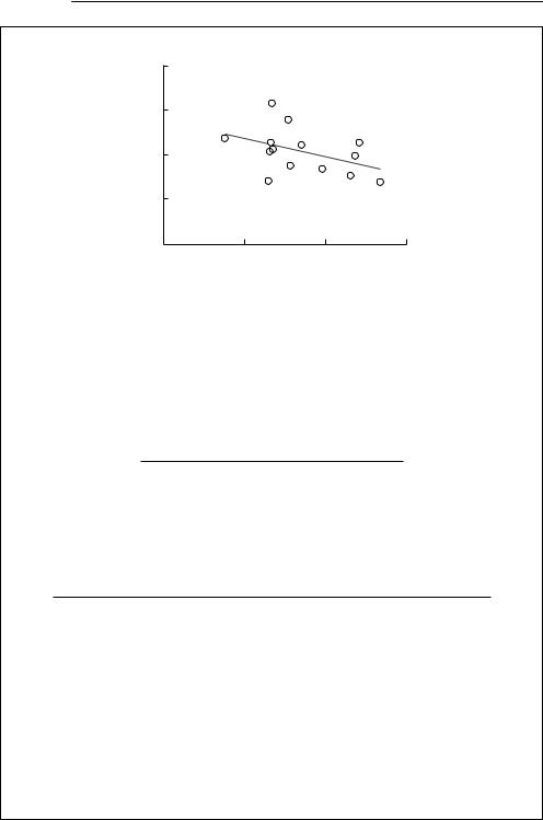
If the percentage surviving to first breeding is plotted versus numbers attempting to breed, there is a suggestion of density-dependent survival (see below), but this tendency is not statistically significant (t = 1.62, 12 df, p = 0.13).
continued on p. 167
D E N S I T Y D E P E N D E N C E 167
Box 6.1 contd
% surviving
40 |
|
|
|
30 |
|
|
|
20 |
|
|
|
10 |
|
|
|
0 |
|
|
|
250 |
300 |
350 |
400 |
No. attempting to breed
However, this approach ignores much of the information in the data, in particular that the numbers of individuals surviving can be considered as the results of a binomial trial. We therefore fitted the following logistic regression model to the data:
|
p |
|
= α + βX , |
|
ln |
|
|
|
|
|
|
|||
1 |
− p |
|
||
where p is the probability of a bird banded as a nestling surviving to first breeding, and α and β are constants. Using GLIM, the following results were obtained.
|
Estimate |
Standard error |
||
|
|
|
|
|
α |
0.178 |
5 |
0.480 |
2 |
β |
−0.004 |
610 |
0.001 |
438 |
|
|
|
|
|
The analysis of deviance table was as follows:
Source |
Deviance |
df |
p |
|
|
|
|
Model |
10.37 |
1 |
0.005 |
Residual |
43.272 |
12 |
0.005 |
Total |
53.637 |
13 |
|
|
|
|
|
There is thus evidence of density dependence, although there is strong evidence of significant residual variation. Residuals for three years (1980, 1981 and 1986) were greater than 2.5, and thus probably outliers. If these are omitted there is still a highly significant effect of numbers attempting to breed on survival ( dev = 8.34, 1 df, p < 0.005) and there is no suggestion of significant residual deviance (dev = 11.58, 9 df ).
168 C H A P T E R 6
Pollard et al. (1987) proposed a broadly similar approach. Their test assumes that the density dependence is a function of the logarithm of current population size, rather than Nt itself. Dennis and Taper (1994) suggest that this will weaken the power of the test to detect density dependence. There is no strong a priori reason to prefer one form of density-dependent function over another, but each could be compared to see how well they represented particular time series. Pollard et al. use a randomization method to test for density dependence. This does not lend itself to placing confidence bands around estimates of the parameters describing density dependence in the way that is permitted by the parametric bootstrap of Dennis and Taper. There is no reason, however, why one should not bootstrap estimates of the parameters from the model of Pollard et al.
These methods are not conceptually particularly difficult, but do involve some computer programming. Fox and Ridsdillsmith (1995) have suggested that the performance of these recent tests as means of detecting density dependence is not markedly better than that of Bulmer (1975). If the objective is to go further and parameterize a model, then Bulmer’s test will not fulfil this need.
In an important series of papers, Turchin and co-workers (Turchin & Taylor, 1992; Ellner & Turchin, 1995; Turchin, 1996) have developed a model which is a generalization of Dennis and Taper’s model. The basic idea is that the logarithm of the finite rate of increase of a population,
|
|
N |
|
|
rt |
= ln |
t |
, |
(6.5) |
|
||||
|
Nt−1 |
|
||
should be a nonlinear function of population density at various lags or delays,
rt = f (Nt−1,Nt−2,Nt−d,εt), |
(6.6) |
where d is the maximum lag in the model, and εt is random noise. The problem is then how best to represent the function f and to estimate its parameters. For moderately short time series (less than 50 data points), Ellner and Turchin (1995) recommend using a response surface methodology which approximates the general function f by a relatively simple polynomial. Specifically, they suggest first power-transforming the lagged population size:
X = Nθ1 . |
(6.7) |
t−1 |
|
This transformation is known as a Box–Cox transformation (Box & Cox, 1964): θ1 = 1/2 corresponds to a square root, θ1 = −1 to an inverse transformation, and θ1 → 0 is a logarithmic transformation.
For a maximum lag of 2 and a second-order polynomial, eqn (6.6) can be written as

D E N S I T Y D E P E N D E N C E 169
r = a |
0 |
+ a |
X + a |
Y + a |
11 |
X 2 |
+ a |
12 |
XY + a |
22 |
Y 2 |
+ ε |
, |
(6.8) |
|
t |
|
1 |
2 |
|
|
|
|
|
t |
|
|
||||
where |
|
|
|
|
|
|
|
|
|
|
|
|
|
|
|
Y = Nθ2 |
. |
|
|
|
|
|
|
|
|
|
|
|
6.9) |
||
|
t−2 |
|
|
|
|
|
|
|
|
|
|
|
|
( |
|
and X is given by eqn (6.7). Higher-order polynomials and longer delays are possible, but require many more parameters to be estimated. Dennis and Taper’s equation (eqn (6.4) ) is a special case of eqn (6.8), with a2, a11, a12 and a22 all 0, and θ1 = 1. Pollard’s model is similar, with θ1 → 0.
The problem now is one of deciding how many terms should be in the model, and to estimate parameters for the terms that are included. As is the case with Dennis and Taper’s method, ordinary least squares is adequate to estimate the aij parameters (but not the power coefficients θ). However, the standard errors, etc. thus generated are not suitable guides to the number of terms that should be included. Again, a computer-intensive method is required. Turchin (1996) suggests a form of cross-validation similar to a jackknife. Each data point is left out in turn, and the model is assessed by its ability to predict this missing data point. The aij parameters are fitted by ordinary least squares, and the values (−1, −0.5, 0, 0.5 and 1) are tried in turn for θ. Full details of the fitting procedure are given by Turchin (1996) and Ellner and Turchin (1995). Commercial software – RAMAS/time (Millstein and Turchin, 1994) – is also available. Box 6.2 shows results from using this approach on a time series for larch budmoth.
In summary, autoregressive approaches to parameterizing density dependence in time series are potentially very powerful. The most general model is eqn (6.6). Most current models are special cases of eqn (6.8). Standard least squares methods are adequate to generate point estimates of parameters, but a computer-intensive method, whether randomization (Pollard et al., 1987), bootstrapping (Dennis & Taper, 1994) or cross-validation (Turchin, 1996), must be used to guide model selection. All models assume white (uncorrelated) noise. This is a major problem (see below), although additional lagged terms may sometimes remove autocorrelation from the residual error. Further progress in this area can be expected in the next few years.
There are inherent problems in attempting to quantify density dependence in any unperturbed time series. All regression-based statistical methods rely on a range of values being available for the predictor variables: the wider the range, the better are the resulting estimates of the regression parameters. In methods that search for density dependence, the predictor variable is population density itself. If the system is tightly regulated, then an unmanipulated population will not vary in density much at all, making the relationship hard to detect. Conversely, if a system is weakly regulated, there will be a range of population densities available on which to base a regression, but the strength

170 C H A P T E R 6
Box 6.2 Analysis of larch budmoth time series
The following analysis is from Turchin and Taylor (1992), and is based on a time series of the larch budmoth Zeiraphera diniana, a forest pest in the European Alps, running from 1949 to 1986. The data shown below are the population density in the upper Engadine Valley, Switzerland, expressed as the logarithm to base 10 of the weighted mean number of large larvae per kilogram of larch branches (digitized from Baltensweiler & Fischlin, 1987).
Year |
Population density |
Year |
Population density |
Year |
Population density |
|||
|
|
|
|
|
|
|
|
|
1949 |
−1.713 |
01 |
1962 |
1.404 |
39 |
1975 |
0.660 |
446 |
1950 |
−1.064 |
18 |
1963 |
2.373 |
45 |
1976 |
−1.905 |
19 |
1951 |
−0.324 |
71 |
1964 |
2.254 |
91 |
1977 |
−2.108 |
36 |
1952 |
0.674 |
519 |
1965 |
0.504 |
905 |
1978 |
−1.266 |
31 |
1953 |
1.867 |
09 |
1966 |
−1.728 |
38 |
1979 |
−0.708 |
14 |
1954 |
2.509 |
89 |
1967 |
−2.614 |
29 |
1980 |
0.991 |
958 |
1955 |
2.107 |
33 |
1968 |
−1.222 |
38 |
1981 |
2.190 |
57 |
1956 |
1.324 |
13 |
1969 |
−0.718 |
68 |
1982 |
2.289 |
5 |
1957 |
0.323 |
372 |
1970 |
0.032 |
79 |
1983 |
1.959 |
49 |
1958 |
−1.076 |
16 |
1971 |
1.019 |
89 |
1984 |
0.765 |
392 |
1959 |
−1.091 |
98 |
1972 |
2.236 |
68 |
1985 |
−0.918 |
11 |
1960 |
−0.406 |
9 |
1973 |
2.408 |
11 |
1986 |
−0.191 |
07 |
1961 |
0.260 |
11 |
1974 |
2.235 |
15 |
|
|
|
|
|
|
|
|
|
|
|
|
Below are the observed data, log-transformed, together with the autocorrelation function (ACF). The ACF is the obtained by correlating the data against itself, at lags shown on the horizontal axis. The maximum of the function at a lag of 9 suggests that the series has a period of that length.
ACF
|
6 |
|
|
|
|
1 |
|
5 |
|
|
|
|
|
t |
4 |
|
|
|
|
|
N |
|
|
|
|
|
|
Log |
3 |
|
|
|
|
0 |
|
|
|
|
|
|
|
|
2 |
|
|
|
|
|
|
1 |
|
|
|
|
|
|
0 |
10 |
20 |
30 |
40 |
–1 |
|
|
|||||
|
|
|
Year |
|
|
|
continued on p. 171
D E N S I T Y D E P E N D E N C E 171
Box 6.2 contd
The parameters obtained by fitting eqn (6.8) to the data are:
θ1 |
θ2 |
a0 |
a1 |
a2 |
a11 |
a22 |
a12 |
0.5 |
0.0 |
− 4.174 |
4.349 |
−1.790 |
−1.280 |
−0.124 |
0.437 |
|
|
|
|
|
|
|
|
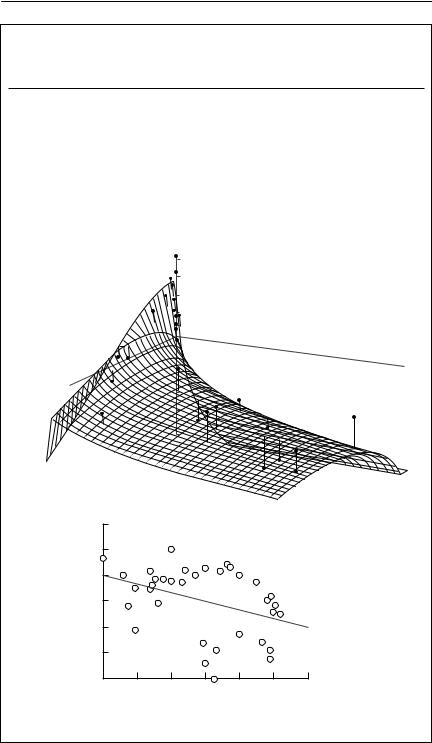
The response surface generated by eqn (6.8) and the above parameters is shown in (a), together with the actual data points. Also shown (b) is the rather confusing relationship between rt and ln Nt−1. It is clear that this particular series requires the second lag term Nt−2.
rt
Nt–2
Nt–1
(a)
rt
(b)
6
4
2
0
–2
–4
1 |
2 |
3 |
4 |
5 |
6 |
|
|
ln Nt–1 |
|
|
|
continued on p. 172
172 C H A P T E R 6
Box 6.2 contd
The reconstructed series is shown below, both without and with noise:
(a) observed series; (b) reconstructed series without random noise; (c) reconstructed series with random process noise, standard deviation σ = 0.2.
|
6 |
|
|
|
|
5 |
|
|
|
t |
4 |
|
|
|
N |
3 |
|
|
|
Log |
|
|
|
|
2 |
|
|
|
|
|
|
|
|
|
|
1 |
|
|
|
(a) |
0 |
|
|
|
|
|
|
|
|
|
4 |
|
|
|
|
3 |
|
|
|
t |
|
|
|
|
N |
2 |
|
|
|
Log |
|
|
|
|
|
|
|
|
|
|
1 |
|
|
|
(b) |
0 |
|
|
|
|
|
|
|
|
|
5 |
|
|
|
|
4 |
|
|
|
t |
3 |
|
|
|
N |
|
|
|
|
Log |
2 |
|
|
|
|
1 |
|
|
|
|
0 |
20 |
30 |
40 |
|
10 |
|||
(c) |
|
Year |
|
|
Note, first, the good correspondence between the observed and reconstructed series; and second, that the series without random noise does not exactly repeat itself. The analysis thus suggests that the series is quasiperiodic. That is, the dynamics are complex, and the period is not a simple integer.
of the relationship is, of course, weak. There will also be substantial problems with observation error bias, if population density is estimated with error. I discuss this bias in more detail in Chapter 11. A common effect of observation error bias is that a relationship that does exist is obscured. Nevertheless, in a study of nearly 6000 populations of moths and aphids caught in light or suction traps in Great Britain, Woiwod and Hanski (1992) found significant

D E N S I T Y D E P E N D E N C E 173
density dependence in most of them, provided sufficiently long time series were used: ‘sufficiently long’ means more than 20 years. It is always going to be difficult to detect and measure density dependence, although it is present, in unmanipulated time series only a few years in length.
A further problem with unmanipulated time series is that they rely on environmental stochasticity to generate the variation in population density. This is almost always assumed to be white noise. In reality, much stochasticity in ecological systems is ‘red’, or highly serially correlated, noise (Halley, 1996; Ripa and Lundberg, 1996). For example, if random, uncorrelated variation in rainfall is used to drive herbivore dynamics via rainfall-dependent vegetation growth, then variation in the resulting herbivore population size is strongly serially correlated – see Caughley and Gunn (1993) or Chapter 9 for more details. Serial correlation may have unpredictable effects on statistical tests for density dependence. For example, a high level of forage will produce high population growth and, if maintained, high population density, obscuring the actual density-dependent effect of food supply (see Chapter 9 for further details).
Demographic parameters as a function of density
An alternative to seeking density dependence in a time series directly is to look for a relationship between either survival or fecundity and density in observed data from a population. Clearly, this requires more information about the population than does a simple analysis of a time series. On the other hand, there are fewer statistical complications, as current population size no longer is part of both response and predictor variables, as it is for time-series analysis. However, the problems with lack of variation in population size in a tightly regulated population, observation error bias in the predictor variable, and autocorrelation in errors are still likely to be present in many cases, particularly if the data come from following a single population through time, rather than from examining a number of replicate populations at differing densities.
Density dependence in fecundity data can normally be looked for using standard regression techniques. An example is Shostak and Scott (1993), which examines the relationship between parasite burden and fecundity in helminths. Individual hosts can be considered as carrying replicate populations of parasites, avoiding the problems of time-series analysis. Survival data are likely to be analysed using logistic regression methods (see Chapter 2, and Box 6.2 for an example).
Experimental manipulation of population density
It should be clear from the previous discussion that there are unavoidable problems with any attempt to describe density dependence from purely

174 C H A P T E R 6
observational data. Manipulative experiments, provided they are not too unrealistic, will almost always provide less equivocal results than purely observational methods. In principle, density may be manipulated either by increasing it beyond normal levels or by experimentally reducing it. The latter approach is to be preferred, because any closed population at all will show either a reduction in fecundity or an increase in mortality or both, if the population is at sufficiently high density. This obvious result does not necessarily shed light on whether density-dependent factors are operating on the population when it is at the densities occurring in the field. On the other hand, an increase in fecundity or decrease in mortality when the population is reduced below normal levels is far more convincing evidence that density dependence operates on natural populations.
Harrison and Cappuccino (1995) review recent experiments on population regulation in which density has been manipulated. Their overall conclusion is that ‘surprisingly few such studies have been done’. Nevertheless, they were able to locate 60 such studies on animal taxa over the last 25 years, and of these 79% found direct density dependence. Most of these studies, however, were concerned solely with determining whether density dependence was present, and could not be used to parameterize a particular functional form to represent density dependence. To do this it is necessary to manipulate the population to several densities, rather than merely to show that there is some relationship between density and demographic parameters.
Experimental manipulation of resources
If density dependence is thought to act via resource limitation, an alternative to manipulating density itself is to manipulate the level of the resources. Several studies have examined the effect of supplementary feeding of wild populations. However, if the objective is to quantify density dependence through describing the relationship between resource level and demographic parameters, it is necessary to include resource dynamics in the model explicitly. This requires the methods described in Chapter 9.
Stock–recruitment relationships
Obtaining a sustained harvest from a population that, without harvesting, is at steady state, relies on the existence of some form of density dependence operating on the population. Otherwise, any increased mortality would drive the population to extinction. It is not surprising, therefore, that detection and parameterization of relationships that quantify density dependence is a major part of fisheries management. Fisheries biologists have usually approached the problem through estimating the form of the stock–recruitment relationship

D E N S I T Y D E P E N D E N C E 175
for exploited species. ‘Stock’ is usually defined as the size of the adult population. Since this needs to be weighted according to the fecundity of each individual, a more precise definition of the average stock size over a short time interval is the total reproductive capacity of the population in terms of the number of eggs or newborn offspring produced over that period (Hilborn & Walters, 1992). Historically, recruits were the individuals reaching the size at which the fishing method could capture them, but ‘recruitment’ can be defined as the number of individuals still alive in a cohort at any specified time after the production of the cohort.
Any stock–recruitment relationship other than a linear relationship passing through the origin implies density dependence of some sort. The simplest possible model in fisheries is the Schaefer model, which assumes logistic density dependence. This is often parameterized by assuming that the population size of the unexploited population is the carrying capacity K. The maximum sustainable yield can then be obtained from the population by harvesting at a rate sufficient to maintain the population at a size of K/2 (see, for example, Ricker, 1975). This very simplistic model is frequently used, despite both theoretical and practical shortcomings (Hilborn & Walters, 1992).
Hilborn and Walters (1992) contains an excellent review of methods for fitting stock–recruitment relationships to fisheries data. The two most commonly used models of stock–recruitment relationships in fisheries are the Ricker model and the Beverton–Holt model. The Ricker model can be written as
R = Sa exp(−bS), |
(6.10) |
where R is the number of recruits, S is stock size, the parameter a is the number of recruits per spawner at low stock sizes, and b describes the way in which recruitment declines as stock increases. The Beverton–Holt model can be written as
R = |
|
aS |
|||
|
|
(6.11) |
|||
|
|
||||
1 |
+ |
a |
S |
||
|
|||||
|
|
|
c |
||
where a has the same meaning as for the Ricker model, and c is the number of recruits at high stock levels. The key distinction between the two models is that the Ricker model allows for overcompensation, whereas the Beverton– Holt model does not.
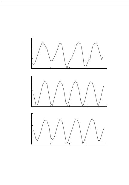
Almost all stock–recruitment data are very variable (see Fig. 6.1), which makes fitting any relationship difficult. It is essential to recognize, however, that variation in the level of recruitment for a given stock size is an important property of the population dynamics, with major implications for management. Such variation is not simply ‘noise’ or error obscuring a ‘true’

176 C H A P T E R 6
4000
Recruits
0
(a)
1000
Recruits
0
(b)
40
Recruits
1600
400
(c) |
0 |
Spawning population size |
25 |
|
|
Fig. 6.1 Examples of Ricker and Beverton–Holt stock–recruitment relationships: (a) Skeena River sockeye salmon; (b) Icelandic summer spawning herring; (c) Exmouth Gulf prawns. In each case, the curve that decreases at high stock size is the Ricker curve, whereas the one that reaches an asymptote is the Beverton–Holt curve. All were fitted using nonlinear least squares on log-transformed data, although the plots shown are on arithmetic axes. The straight dashed line on the Skeena River relationship is the line along which stock equals recruitment. In a species which reproduces only once, such as this salmon, the intersection of the line with the stock–recruitment line gives the equilibrium population size. The line has no particular meaning for species that may reproduce more than once, so it is not shown on the other two figures. Note the amount of variation in each relationship. From Hilborn and Walters (1992).
3
Recruits
0
(a)
3
Recruits
0
(b)
|
|
|
D E N S I T Y D E P E N D E N C E 177 |
|
Observed |
3 |
|
Observed |
|
|
||||
|
|
|||
|
|
|
|
|
|
|
|
|
|
1.5 |
0 |
1.5 |
||||
|
Actual |
3 |
|
Actual |
||
|
|
|||||
|
|
|
||||
|
|
|
|
|
|
|
|
|
|
|
|
|
|
Spawners |
1.5 |
0 |
Spawners |
1.5 |
|
|
|
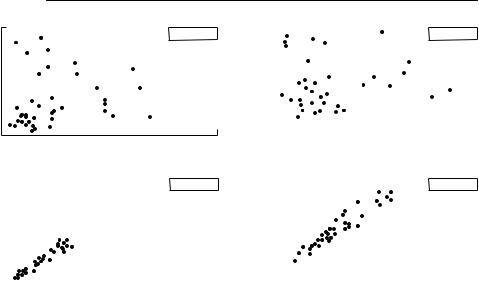
Fig. 6.2 Simulated relationships between estimated stock size S and estimated recruitment R with observation error: (a) observed relationship, and (b) actual relationship without observation error. These relationships were generated from the simple stock– recruitment equation Rt+1 = Rt(1 − Ht) exp(α + ut), where Rt is the number of recruits in generation t, Ht is a harvest level (assumed to be fairly high), α is a measure of the intrinsic
growth rate, and ut is a random normal deviate, to simulate process noise. The number of recruits is measured with lognormal observation error, such that Ot = Rt exp(νt), where Ot is the observed recruitment, and νt is a random normal deviate. In both of these examples,
σ 2u = 0.1 and σ 2ν = 0.25. From Walters and Ludwig (1981).
relationship. It an essential part of the stock–recruitment relationship and needs to be quantified and taken into account, not eliminated. As well as such process error, there is also likely to be substantial observation error. The observed stock and recruitment levels are estimates only of the true levels, and are usually quite imprecise. Observation error is discussed in Chapter 2. It is particularly a problem when it occurs in the predictor variable, which in this case is the stock size. Unless the error in the estimation of stock size is much smaller than the amount of variation in actual stock size, it will be quite impossible to detect a stock–recruitment relationship. This point is illustrated using a simple simulation in Figure 6.2. In Chapter 11, I discuss some approaches that may prove useful in dealing with observation error in predictor variables.
In the face of these problems, Hilborn and Walters’s (1992) advice is as follows:
1 Any fitted stock–recruitment curve is at best an estimate of the mean relationship between stock and recruitment, not an estimate of a true relationship. The true relationship includes variation around the mean.
178 C H A P T E R 6
2 The process error in recruitment size can be expected to have an approximately lognormal distribution. This means that to obtain maximum likelihood estimates of parameters, recruitment should be log-transformed before least squares methods are applied.
3 Asymptotic confidence intervals, as generated by standard nonlinear estimation packages, are likely to be quite unreliable, both because of the level of variation present, and because of the likelihood of strong correlations between parameter estimates. Computer-intensive methods such as bootstrapping or jackknifing (see Chapter 2) are needed.
4 Observation error is likely to obscure the relationship between stock and recruitment. If the size the error is known or estimated from independent data, it can be corrected for to some extent (see Chapter 11; or Ludwig & Walters, 1981). Otherwise, it is worth using simulation with plausible estimates to explore the possible consequences of observation error.
5It is always worth looking at residuals.
More sophisticated methods of estimating stock–recruitment relationships
can be considered as density-manipulation experiments, in which the varying harvest levels are used to alter density, although there are rarely controls or replications. This idea has been formalized as ‘active adaptive management’ (Smith & Walters, 1981), in which harvest levels are deliberately varied in order to obtain information about the nature of the stock–recruitment relationship.
Further complications
Stochasticity
It is very clear that density dependence does not always act in a predictable way on a given population. For example, where density dependence acts through food limitation, the amount of food available to a population will vary according to environmental conditions. Where density dependence acts through a limited number of shelter sites from which to escape harsh weather, the level of mortality imposed on individuals in inadequate shelter will depend on the harshness of the weather. This fairly obvious concept has been labelled ‘density-vagueness’ (Strong, 1986).
To include such stochastic density dependence in a mechanistic model, it is necessary not only to find parameters and a functional form capable of representing the mean or expected level of density dependence at any given population size, but also to describe the probability distribution of density dependence at any given population size. This will never be easy, given the proliferation of parameters that is required.
The most general and flexible approach, but the one most demanding of data, is to use a transition-matrix approach. Getz and Swartzman (1981) took

D E N S I T Y D E P E N D E N C E 179
Table 6.3 A transition matrix for a stochastic stock–recruitment relationship. This example is for a purse-seine anchovy fishery off South Africa. The stock data were divided into eight levels, and the recruitment into seven levels. Each element in the table is the probability of a given stock level producing a particular recruitment level. From Getz and Swartzman (1981)
Recruitment level j
High
← →
Low
|
Low |
← |
Stock level i |
→ |
High |
||||
|
|
|
|
|
|
||||
|
1 |
2 |
3 |
4 |
5 |
6 |
7 |
8 |
|
7 |
0.0 |
0.05 |
0.05 |
0.05 |
0.05 |
0.05 |
0.05 |
0.05 |
|
6 |
0.0 |
0.05 |
0.1 |
0.1 |
0.15 |
0.2 |
0.25 |
0.25 |
|
5 |
0.05 |
0.1 |
0.15 |
0.25 |
0.30 |
0.35 |
0.35 |
0.35 |
|
4 |
0.15 |
0.2 |
0.35 |
0.3 |
0.25 |
0.2 |
0.2 |
0.2 |
|
3 |
0.15 |
0.4 |
0.25 |
0.25 |
0.2 |
0.15 |
0.1 |
0.1 |
|
2 |
0.45 |
0.15 |
0.1 |
0.05 |
0.05 |
0.05 |
0.05 |
0.05 |
|
1 |
0.2 |
0.05 |
0.0 |
0.0 |
0.0 |
0.0 |
0.0 |
0.0 |
|
|
|
|
|
|
|
|
|
|
|
extensive data sets on stock size and resulting recruitment levels, and grouped both stock and recruitment data into six to eight levels. They then calculated the frequency with which stock level i gave rise to recruitment level j, producing transition matrices like the one shown in Table 6.3. This method of generating a stock–recruitment relationship is entirely flexible, allowing for any form of density dependence whatsoever, and allows the probability distribution of recruitment for a given stock size to take any form consistent with the data. However, it requires the estimation of as many parameters as there are elements in the transition matrix (at least 42 in the examples Getz and Swartzman discuss), and cannot be expected to be reliable without some hundreds of data points.
An approach less demanding of data is simply to use the variance estimate generated by a standard least squares regression to add stochasticity to a simulation. As is mentioned above, it is often reasonable to assume that ‘abundance’ has an approximately lognormal error. If this is the case, least squares regression on log-transformed data produces maximum likelihood estimates of the model parameters. This is the case whether the regression is linear or nonlinear. A maximum likelihood estimate of the variance of the error of the log-transformed data can then be obtained from
F2 = |
SSE |
, |
(6.12) |
|
|||
|
n − p |
|
|
where SSE is the error (residual) sum of squares, n is the number of data points and p is the number of parameters fitted. This can then be used in simulations. If there is substantial observation error in either dependent or predictor variables or both, this approach may not work well.
A final approach is to model the process producing the density dependence, and to introduce stochasticity into that model. For example, Chapter 9

180 C H A P T E R 6
discusses a model in which a herbivore is limited by food supply, and plant growth is driven by stochastic rainfall. This approach probably produces the best representation of stochastic density dependence, but at a cost of adding a level of additional complexity.
Inverse density dependence
Most discussions of density dependence concentrate, as has this chapter, on direct density dependence. There is also the possibility of inverse density dependence, in which survival and/or fecundity increase as density increases. The phenomenon is often called an Allee effect. In the fisheries literature, inverse density dependence is usually called depensation. Inverse density dependence may be of considerable applied importance. If it occurs at low population densities, there may be a minimum population density below which the population will decline to extinction, because the mean death rate exceeds the mean birth rate. If it occurs at higher population densities, population outbreaks are likely to occur. It may be of particular importance when attempting to predict the rate of spread of an invading species. For example, Veit and Lewis (1996) found that it was necessary to include an Allee effect in a model of the house finch invasion of North America. Otherwise, the qualitative features of the pattern of spread could not be reproduced. However, they were unable to estimate the size of the effect from the available data, other than by choosing the value for which their predicted rate of population spread most closely approximated the observed rate of spread.
A variety of mechanisms have been suggested that may produce inverse density dependence. Allee’s original idea (Allee et al., 1949) was that, when a population becomes very sparse it is difficult for animals to locate mates. Other possibilities are that group-based defences against predators might be compromised at low population densities, or that foraging efficiency might be reduced (Sæther et al., 1996).
Inevitably, inverse density dependence is difficult to detect or quantify in the field. Because it is expected to be a characteristic of rare populations, it will always be hard to obtain adequate data for reliable statistical analysis, and the effects of stochasticity will be considerable. Nevertheless, there have been several attempts to investigate it systematically.
Fowler and Baker (1991) reviewed large mammal data for evidence of inverse density dependence, including all cases they could find in which populations had been reduced to 10% or less of historical values. They found no evidence of inverse density dependence, but only six studies met their criterion for inclusion in the study of a 90% reduction in population size. Sæther et al. (1996) applied a similar approach to bird census data, obtaining 15 data sets satisfying the criterion that the minimum recorded density was 15% or

D E N S I T Y D E P E N D E N C E 181
less of the maximum density recorded. They then used a quadratic regression to predict recruitment rate, fecundity or clutch size as a function of population density. Their expectation was that an Allee effect would produce a concave relationship between the recruitment rate and population density, so that the coefficient on the quadratic term would be positive. In all cases, however, they found that a convex relationship better described the data. A limitation of this approach is that, assuming an Allee effect, one might expect a sigmoidal relationship between recruitment and population size over the full range of population size (direct density dependence would cause a convex relationship at high population densities). If most of the available data are at the higher end of the range of population densities, then the directly density-dependent component of the curve would dominate the relationship.
Myers et al. (1995) have produced the most complete analysis of inverse density dependence in time-series data. They analysed stock–recruitment relationships in 128 fish stocks, using a modified Beverton–Holt model,
R = |
αSδ |
|
1 + Sδ/K . |
(6.13) |
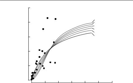
Here, R is the number of recruits, S is the stock size, and α, K and δ are positive constants (compare with eqn (6.11)). If there is inverse density dependence, δ > 1, as is shown in Fig. 6.3. Myers et al. (1995) fitted eqn (6.13) by nonlinear regression to log-transformed recruitment. (To reiterate, this process corresponds to using maximum likelihood estimation, if the variation is lognormal.) They found evidence of significant inverse density dependence in only three cases. This approach may lack power, if few data points are at low population densities. Myers et al. used a power analysis, which showed that in 26 of the 128 series, the power of the method to detect δ = 2 was at least 0.95. The results suggest that depensation is not a common feature of commercially exploited fish stocks.
Liermann and Hilborn (1997) reanalysed these same data from a Bayesian perspective. They suggest that the δ of eqn (6.13) is not the best way to quantify depensation, because the amount of depensation to which a given δ corresponds depends on the values taken by the other parameters. As a better measure, they propose the ratio of the recruitment expected from a depensatory model to that expected from a standard model, evaluated at 10% of the maximum spawner biomass. Using this reparameterization, they show that the possibility of depensation in four major taxa of exploited fish cannot be rejected.
Comparing the conclusions reached by Liermann and Hilborn (1997) with those arrived at by Myers et al. (1995), from precisely the same data set makes two important and general points about parameter estimation. First, reparameterizing the same model and fitting it to the same data can produce
182 C H A P T E R 6
|
25 |
|
|
20 |
|
) |
|
|
12 |
|
|
10 |
15 |
|
(x |
||
|
||
Recruitment |
10 |
|
|
5
0
δ =2 δ =1.8 δ =1.6 δ =1.4
δ =1.2 δ =1
0 |
2 |
4 |
6 |
8 |
10 |
12 |
Spawner biomass (x 106 metric tons)
Fig. 6.3 Inverse density dependence in a Beverton–Holt stock–recruitment model. The dots are actual recruitment data for the California sardine fishery, and the heavy solid line is the standard Beverton–Holt model (eqn (6.11)) fitted to the data. The light solid lines show how this estimated curve is modified by using eqn (6.13), with varying values of δ. The parameters of each of these curves were chosen so that they have the same asymptotic recruitment as the fitted curve, and so that they have the same point of 50% asymptotic recruitment. From Myers et al. (1995).
different results: to make biological sense of modelling results, it is important that parameters should have direct biological or ecological interpretation. Second, reinforcing a point made in Chapter 2, conventional hypothesistesting approaches give logical primacy to the null hypothesis. That is, they assume that a given effect is not present, in the absence of strong evidence that it is present. For management purposes, such as the prudent management of fish stocks, giving logical primacy to the null hypothesis may not be sensible. As Liermann and Hilborn suggest, a Bayesian approach may be more appropriate.
As with any other ecological process, manipulation is likely to be a more satisfactory way to detect an Allee effect than is observation. Kuusaari et al. (1998) report one of the few manipulative experiments on Allee effects in the literature. They introduced differing numbers of Glanville fritillary butterflies (Melitaea cinxia) to empty habitat patches, and found a significant inverse relationship between population density and emigration rate, even after patch area and flower abundance had been controlled for. They also found a positive relationship between the proportion of females mated and local population density in unmanipulated populations.

D E N S I T Y D E P E N D E N C E 183
Summary and recommendations
1 Density dependence is difficult to detect and quantify in natural populations, but its omission will cause many mechanistic models to fail.
2 Adjusting survival and fecundity estimates so that r = 0 and omitting density dependence produces estimates of extinction risks that will lead to conservative management actions, provided that the omitted density dependence is direct. This approach is useful over moderate time horizons. However, it will not produce useful estimates of extinction risks if the objective is to investigate the impact of additional mortality, such as harvesting.
3 Models based on the logistic equation require an estimate of the ‘carrying capacity’ of a population. This is the population level beyond which unspecified density-dependent factors will cause the population growth rate to be negative. It is not the peak population size ever attained.
4 A variety of nonlinear time-series methods are now available to produce a statistically rigorous framework for studying density dependence in time series. Obtaining point estimates using these approaches is relatively straightforward, but standard regression packages cannot be used to perform tests of significance or to estimate standard errors. Computer-intensive methods such as bootstrapping need to be used. Even these methods are unreliable if there is substantial observation error, or if there is autocorrelated ‘red’ process error.
5 It is easier to quantify density-dependent effects on demographic parameters than it is to quantify density dependence in a time series itself. However, if the population density or population size is estimated imprecisely, this observation error will tend to obscure density dependent effects.
6 Manipulative experiments are usually a better way to quantify density dependence than is simple observation. If your objective is to show that density dependence is important in a natural situation, it is better to reduce the natural population density than to augment it artificially.
7 Density dependence or ‘compensation’ must occur if a population is to be harvested sustainably. Fisheries biologists usually quantify it by using a stock–recruitment relationship, fitting one of two standard models: the Ricker or Beverton–Holt. Specific advice on applying these is provided earlier in the chapter.
8 Stochasticity is an essential feature of density dependence, but is difficult to deal with.
9 Inverse density dependence at low population density may be very important, particularly in conservation biology. It is difficult to detect and quantify, because it occurs when animals are rare. It can potentially be quantified using a modified stock–recruitment relationship. A more powerful approach is to investigate inverse density-dependent effects on particular demographic parameters.