Host–pathogen and host–parasite models

H O S T – P A T H O G E N A N D H O S T – P A R A S I T E M O D E L S 285

brushtail possum (Trichosurus vulpecula). Pathogens, or less commonly, parasites (McCallum & Singleton, 1989), may be considered as control agents for problem species. Models can be used to evaluate the likelihood of successful control (e.g. Barlow, 1997) or the optimal timing of release of the agent (e.g. McCallum, 1993). The objective of modelling may also be to determine the possible impact of infection on a given species, particularly if the species is of value as game (see, for example, Hudson & Dobson, 1989), or if the species is endangered (McCallum & Dobson, 1995).

The models that are required for such problems can span the range from strategic to tactical, as is discussed in the introductory chapter. A particularly important consideration in parameter estimation is whether the model is intended to be applied to the same system in which the parameter has been estimated. For example, Woolhouse and Chandiwana (1992) estimated the rate of infection of snails with Schistosoma mansoni in Zimbabwe, with the objective of using the estimated parameter to model the dynamics of the disease in that same area. If the objective of modelling is to predict the possible impact of an exotic disease, or a novel biocontrol agent, then it is clearly impossible to estimate the parameter in the environment in which the model is to be applied. The problems of extrapolation from laboratory studies to the field, or from one field situation to another, are considerable, particularly for the key process of transmission.

Basic structure of macroparasite and microparasite models

For modelling purposes, it is convenient to divide parasites into microparasites, which usually can reproduce rapidly within their hosts, and macroparasites, which usually must leave their host at some point in a complete life cycle. A virus or bacterium is a typical microparasite, and a helminth is a typical macroparasite. The simplest models of microparasitic infections consider hosts as ‘infected’, without attempting to differentiate between degrees of infection. As the microparasite can reproduce rapidly within its host, the level of infection depends primarily on the level of host response, rather than on the number of infective stages the host has encountered. In contrast, the impact of a macroparasitic infection on its host depends quite critically on the number of parasites the host is carrying, which depends in turn very strongly on the number of infective stages encountered. It is thus essential, even in the simplest models, to keep some track on the distribution of parasites between hosts. These generalizations are oversimplifications: recent research has emphasized the importance of the infective dose on the severity of disease in microparasites and the importance of host response to the level of infection in macroparasitic infections (Anderson & May, 1991). Nevertheless, they provide a point at which to start.

286 C H A P T E R 1 0

Models of microparasitic infections

Most recent models are based on the framework outlined by Anderson and May (1979) and May and Anderson (1979). This is, in turn, based on earlier models (Ross, 1916; 1917; Bailey, 1975), dating back to Bernoulli (1760). For ecologists, the major advance in Anderson and May’s models is that the host population is dynamic and influenced by the disease, so that the ability of a disease to regulate its host population can be examined.

The basic model structure involves dividing the host population into three categories: susceptibles, infecteds and resistants. These models are often therefore called SIR models. Anderson and May use the variables X, Y and Z to identify these categories, respectively. Hosts in each category are assumed to have a per capita birth rate of a per unit of time, and to die at a diseaseindependent rate b. The death rate of infected hosts is augmented by a factor α. Infection is assumed to occur by direct contact between infected and naïve hosts by a process of simple binary collision. This means that hosts leave the susceptible class and enter the infected class at a rate βXY. Infected hosts recover to enter the resistant class at a rate γ per unit of time. Finally, resistance is lost at a rate ν per unit of time.

These assumptions lead to the following equations:

The full details of the behaviour of this model can be found in Anderson and May (1979) and May and Anderson (1979), and some of the many elaborations of the model are discussed in Anderson and May (1991). Two fundamental and related quantities can be derived from the model. These are the basic reproductive number of the disease, R0, and the minimum population size for disease introduction, NT. Estimation of these quantities, either directly or as compounds of other parameters, is often essential to predict the behaviour of a disease in a population.

The basic reproductive number is the number of secondary cases each primary infection gives rise to, when first introduced into a naïve population. If R0 > 1, the disease will increase in prevalence, but if R0 < 1, the disease will die out. In almost all disease models, R0 depends on the population density, and NT is the critical host population size at which R0 = 1.

H O S T – P A T H O G E N A N D H O S T – P A R A S I T E M O D E L S 289

There is also a threshold host population for parasite introduction:

This makes it clear that parasite reproduction must exceed parasite death (the first term in the denominator). Otherwise there is no host density at which the parasite will persist, but once this occurs, the higher the transmission rate relative to the death rate of the infective stages, the lower the host density at which the infection can persist.

This model is a vast oversimplification of the dynamics of most macroparasite infections. Many macroparasites have complex life cycles with one or more intermediate hosts. This can be accommodated by coupling two or more sets of these basic equations together (Roberts et al., 1995). Infection rates may depend on the age of the host, or infection may occur as a process more complex than binary collision. Parasites may affect host fecundity as well as mortality, and the death rate may not be a simple linear function of burden. Host death may not lead to parasite death. The model also does not include any effects of density dependence within the individual host, either on production of infective stages or on the death rate of parasites within hosts.

Nevertheless, this very simple model identifies clearly the key processes that must be quantified to understand a host–macroparasite infection. They are the infection process, the production of transmission stages, the effect of parasites on hosts, and the loss rate of parasites on hosts. The reproductive number R0 and the threshold host population HT are also of crucial importance. The important distinction between macroparasite and microparasite infections is that, for macroparasites, it is vital to consider the effect of the parasite burden of a host, not simply whether or not it is infected. At a population level, it is essential to quantify the nature of the parasite distribution between hosts, and not simply to measure the mean burden.

The transmission process

The rate at which disease is transmitted between hosts, or the rate at which infective stages infect hosts, is obviously of central importance in determining whether and how fast a disease or parasite will spread in a population (see eqns (10.4) and (10.12) ). It is, however, a particularly difficult process to quantify in the field. Unfortunately, it is also very difficult to apply the results of experiments on laboratory or captive populations to the field. Transmission involves at least two distinct steps. First, there must be contact between the

290 C H A P T E R 1 0

susceptible host and the infective stage, infected host or vector. Second, following contact, an infection must develop, at least to the point that it is detectable, in the susceptible host. Most methods of estimating transmission rates confound these two processes.

Force of infection

In general terms, the quantity that needs to be measured is the force of infection, which is the rate at which susceptible individuals acquire infection. In principle, the force of infection can be estimated directly by measuring the rate at which susceptible individuals acquire infection over a short period. The usual approach is to introduce ‘sentinel’ or uninfected tracer animals; these are removed after a fixed period and their parasite burden (for macroparasites) or the prevalence of infection in the sentinels (for microparasites) determined. This has been done in a number of studies (Scott, 1987; Quinnell, 1992; Scott & Tanguay, 1994), although none of these used an entirely unrestrained host population.

In practice, estimating the force of infection by using sentinels in a natural situation is not a straightforward task. First, it is necessary to assume that the density of infected hosts or parasite infective stages remains constant over the period of investigation. Second, if sentinels are animals that have been reared in captivity, so that they can be guaranteed to be parasite-free, it is most unlikely that, once released, they will behave in the same way as established members of the wild population. The extent of their exposure to infection may therefore be quite atypical of the population in general. If they are members of the wild population that have been selected as sentinels because they are uninfected, then they clearly are not a random sample of the whole population with respect to susceptibility or exposure to infection. The force of infection will therefore probably be underestimated. Finally, if sentinels are wild animals that have been treated to remove infection, there is the possibility of an immune response influencing the results.

A similar approach to using sentinels is to use the relationship between age of hosts and prevalence of infection (microparasites) or parasite burden (macroparasites) to estimate force of infection. Here, newborns are essentially the uninfected tracers. This approach has been used with considerable success in the study of human infections (Anderson & May, 1985; Grenfell & Anderson, 1985; Bundy et al., 1987). In the simplest case, the force of infection is assumed to be constant through time and with age. Then, in the case of microparasitic infection,

H O S T – P A T H O G E N A N D H O S T – P A R A S I T E M O D E L S 291

where x is the proportion of susceptible individuals of age a and Λ is the force of infection. Equivalently,

where F is the proportion of a cohort that has experienced infection by age a (Grenfell & Anderson, 1985). This equation means that Λ is simply the reciprocal of the average age at which individuals acquire infection (Anderson & Nokes, 1991). Unfortunately, the force of infection will rarely be independent of age or time. Methods are available to deal with the problem of age dependence (Grenfell & Anderson, 1985; Farrington, 1990), provided either age-specific case notification records or age-specific serological records are available. If age-specific serological records are available at several times, it may even be possible to account simultaneously for both time and age-specific variation in the force of infection (Ades & Nokes, 1993). Age-specific serology is more likely than age-specific case notifications to be available for nonhuman hosts, but it will not give an accurate picture of age at infection if there is substantial disease-induced mortality. Use of age-specific serology in wildlife also presupposes the age of the animals can be estimated accurately.

For macroparasites, the equation equivalent to eqn (10.14) is

where M is the mean parasite burden at age a and μ is the death rate of parasites on the host. Equation (10.16) has a solution

The force of infection can therefore be estimated from the asymptote of the relationship between mean parasite burden and age, provided an independent estimate of the parasite death rate is available. It is possible to generalize these results to cases in which either the force of infection or parasite death rate varies with the age of the host (Bundy et al., 1987).

There are few cases in which age-specific prevalence or intensity of infection has been used to estimate the force of infection in wildlife. Two notable examples are the study of transmission of the nematode Trichostrongylus tenuis in the red grouse Lagopus lagopus scoticus by Hudson and Dobson (1997), and the study of force of infection of schistosome infections in snails by Woolhouse and Chandiwana (1992). These examples demonstrate that age-prevalence or age-intensity data are potentially powerful tools to estimate the force of infection in natural populations.

294 C H A P T E R 1 0

Experimental estimation of transmission

Several studies have attempted to quantify transmission in macroparasites under experimental conditions (Anderson, 1978; Anderson et al., 1978; McCallum, 1982a). The process occurring in an experimental infection arena can be represented by the following two equations, for the infective-stage population size W and parasite population on hosts P (McCallum, 1982a):

Here, μ is the death rate of the infective stages, s is the proportion of infections that successfully develops into parasites, and H is the number of hosts present. The remainder of infection events remove the infective stage from the system, but a parasite infection does not result.

Equations (10.18) and (10.19) have a time-dependent solution,

Simple infection experiments thus do not produce a straightforward estimate of β, unless the exposure time is very short, in which case eqn (10.20) is approximately

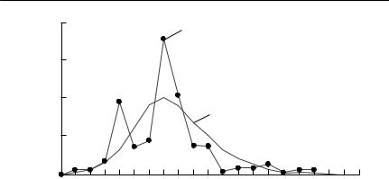
If a constant number of hosts is exposed to varying numbers of infective stages until all infective stages are dead, eqn (10.20) also predicts that a relationship of the form P = kHW will result, but the constant k is s/(μ/β + H), not β itself. In general, to estimate β, it is necessary to use several exposure times and to have an independent estimate of μ. An example of an experiment of this type (from McCallum, 1982a) on the ciliate Ichthyophthyrius multifiliis infecting black mollies (Poecilia latipinna) is shown in Fig. 10.3.

Estimating transmission rates from an observed epidemic

When a disease is introduced into a naïve population (a population without recent prior exposure to the disease) which exceeds the threshold population size, an epidemic results, in which the number of new cases per unit of time will typically follow a humped curve. If there are no new entrants into the susceptible class (either by recruitment or loss of immunity), the epidemic will cease. If a satisfactory model is developed to describe the host–pathogen

Week ending

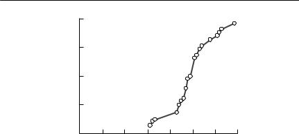
Fig. 10.5 Observed and predicted epidemic curves for phocine distemper in common seals (Phoca vitulia) in The Wash, UK, in 1988. From Grenfell et al. (1992).

considerably between colonies. Serological evidence suggested that it was the transmission rate that varied. This example emphasizes that transmission rates estimated for a given host–pathogen interaction in one place cannot easily be applied to the same interaction in another place. An example of observed and predicted epidemic curves obtained for phocine distemper is shown in Fig. 10.5.

Allometric approaches

It should be clear that direct estimation of the transmission rate is difficult. De Leo and Dobson (1996) have suggested a method based on allometry (scaling with size), which can be used in the absence of experimental data. As with any allometric approach to parameter estimation (see also Chapter 5), it should be considered a method of last resort. It does, however, permit a minimum plausible transmission rate to be estimated to the correct order of magnitude.

For any given epidemic model, it is possible to calculate a minimum transmission rate, which must be exceeded if a disease is able to invade a population of susceptible hosts at a particular carrying capacity. For example, De Leo and Dobson (1996) show that, for a model of the general form of eqns (10.1)–(10.3),

where α is the disease-induced death rate, b is the disease-free host death rate, γ is the recovery rate and K is the carrying capacity in the absence of infection. There are well-established relationships between body size and both

298 C H A P T E R 1 0

carrying capacity and lifespan in vertebrates (see Peters, 1983). As any disease that exists in a given species must be able to invade a fully susceptible population, eqn (10.24) can be combined with these allometric relationships to generate the minimum transmission rate for a disease with a given mortality rate to persist in a host species with a mean body weight w:

Here, m is the factor by which the disease-induced death rate exceeds the disease-free death rate (i.e. m = α/b).

Similar relationships can be derived for other host–microparasite models (see De Leo & Dobson, 1996).

Scaling, spatial structure and the transmission rate

Applying an estimate of a transmission rate obtained in one situation (perhaps an experimental arena) to another situation (perhaps to a field population) is not straightforward. The binary collision model assumed in eqn (10.2) or eqn (10.7) is an idealization borrowed from the physical sciences (de Jong et al., 1995), and is at best a very crude caricature of interactions between biological organisms. As I have said earlier, transmission of infection depends on at least two processes: contacts between susceptible hosts and infectious hosts or stages, and the successful establishment of infection following contact. Equation (10.20) shows how these processes can be separated in some experimental situations. In natural or semi-natural populations, this will rarely be possible. It is the contact rate that causes problems in scaling.

The binary collision model assumes that infected and susceptible animals contact each other randomly and instantaneously, as if they were randomly bouncing balls in a closed chamber. This means that the probability of a contact between a particular susceptible individual and any infected individual is proportional to the density of infected individuals per unit area or volume. De Jong et al. (1995) describe this assumption as the ‘true mass-action assumption’. If transmission is indeed being considered within an arena of fixed size, and all individuals move randomly throughout the arena, then the probability of contact between a susceptible individual and any infected individual is also proportional to the number of infected individuals. It does not matter whether the equations are formulated in terms of density per unit area or number of individuals. Real populations do not live in arenas, and herein lies a problem.

Equations (10.1)–(10.3) are usually presented with X, Y and Z representing population sizes, not densities per unit area. De Jong et al. (1995) argue that, if density remains constant, independent of population size, the term βXY in eqn (10.2) does not represent ‘true mass action’. If population density is constant, but the actual population size varies, the total number of contacts per unit of time made by a susceptible individual will be constant, and the

H O S T – P A T H O G E N A N D H O S T – P A R A S I T E M O D E L S 299

probability of infection will depend on Y/N, the proportion of those contacts which are with infected individuals. Thus, they argue that, for ‘true mass action’ βXY should be replaced by βXY/N, and that βXY represents ‘pseudomass action’. Reality probably lies somewhere between these two. Individuals do not interact equally with all members of their population, but do so mostly with their near-neighbours. This means that local population density is the key variable to which transmission is probably proportional. For most animals, an increase in total population size will increase local population density, but territorial or other spacing behaviour is likely to mean that the increase in density is not proportional to overall population size, unless the population is artificially constrained. A possible empirical solution might be to use a transmission term of the form βXY/Nα, where 0 < α < 1 is a parameter to be estimated.

There is little empirical evidence available to distinguish between these two models of transmission. Begon et al. (1998) used two years of time-series data on cowpox infection in bank voles (Clethrionomys glareolus) in an attempt to resolve whether pseudoor true mass action better predicted the dynamics of infection. Models of transmission based on pseudo-mass action performed marginally better, but the results were inconclusive. One conclusion was, however, clear. The study used two separate populations, and whether pseudoor mass action was assumed, the estimated transmission parameter differed substantially between the two populations. This emphasizes the difficulty of applying a transmission rate estimated in one place to another.

The terms ‘pseudo-’ and ‘true’ mass action are potentially confusing. De Leo and Dobson (1996) consider the same two models, but use the term ‘densitydependent transmission’ for a transmission term βXY, and ‘frequencydependent transmission’ for a transmission term βXY/N. This terminology is less ambiguous.

The rather unsatisfactory conclusion to the scaling problem is that there is really no way that an estimate based on experiments in a simple, homogeneous arena can be applied to a heterogeneous, natural environment. There is simply too much biological complexity compressed into a single transmission term. The best suggestion that can be made is to deal with densities per unit area, rather than actual population size. If this is done, then the coefficient β is not dimensionless: it will have units of area per unit of time.

Parasite-induced mortality

As discussed in Chapter 4, mortality or survival in captive situations is rarely a good indication of mortality in the field, but mortality in the field is not an easy thing to measure. These problems also, of course, apply to attempts to estimate parasite-induced mortality, but are exacerbated because parasites frequently affect host behaviour, possibly leading to increased exposure to predation

300 C H A P T E R 1 0

or decreased foraging efficiency (Dobson, 1988; Hudson et al., 1992a). Experimental infections of animals in laboratory conditions will almost always underestimate disease-induced mortality rates in the field, but field data will not be easy to obtain.

The ‘ideal experiment’

In principle, the best way to obtain such data would be to capture a sample of animals from a population in which the parasite or pathogen does not occur, to infect some with known doses of the pathogen or parasite, to sham-infect others to serve as controls and then to release them and monitor survival. The resulting data could then be analysed using standard survival analysis techniques, treating infection as a covariate (see Chapter 4). This approach has rarely been used, for several reasons. If the pathogen is highly transmissible, the controls may become infected. There are obvious ethical problems in experimentally infecting wild animals, particularly if the study species is endangered. Even if this could be done, there are also difficulties in relating the parasite burden established on the treated animals to the infective dose given to them. All statistical models that attempt to estimate a parameter as a function of a predictor variable produce a biased parameter estimate, if the predictor is measured with error. Some methods to deal with this problem are discussed in Chapter 11.

Comparing survival of hosts treated for infection with controls

Rather than infecting uninfected hosts, an alternative approach is to treat some hosts for the infection, and then to compare survival between these and control hosts. This is obviously an easier approach to justify ethically. A number of studies have used this approach (e.g. Munger & Karasov, 1991; Gulland, 1992; Hudson et al., 1992b), but usually with the objective of determining whether the parasite or pathogen has any impact, rather than quantifying the extent of impact.

There are several design issues that should be addressed if this approach is to be successful. Some of these are standard principles of experimental design, such as appropriate replication and controls. The process of capture and administration of the treatment may well have impacts on survival and behaviour, and, as far as possible, these impacts should be the same for both treatments and controls. Others are specific to experiments of this type. For example, it is important to have some idea of the infection status of each experimental animal before the manipulation takes place.

In a microparasite infection, if only a fraction of the untreated animals are infected in the first place, then the impact of the disease on survival will be

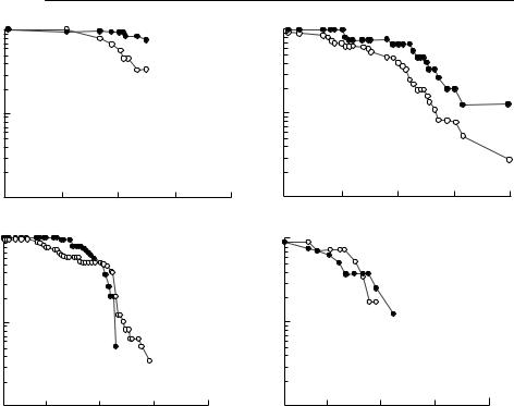
Fig. 10.6 Daily survival rates of anthelminthic-treated and control Soay sheep (Ovis aries) on St Kilda, Scotland, during a population crash in 1989. The x axis shows the time in days from when the first dead sheep was found, and the y axis shows the probability of survival on a logarithmic scale: (a) ewes, χ 2 for difference in daily survival 4.26, 1 df, p < 0.05; (b) male lambs, χ 2 for difference in daily survival 4.57, 1 df, p < 0.05; (c) yearling males, χ 2 for difference in daily survival 0.0, 1 df, not significant; (d) two-year-old males, χ 2 for difference in daily survival 0.1, 1 df, not significant. From Gulland (1992).

underestimated by the experiment. Ideally, one would want to perform a twoway experiment, with infection status before the experiment crossed with treatment. Less obviously, if there is a treatment effect, survival will be more variable in the untreated group than in the treated group, because only some of the untreated group will be infected. This will produce problems for most statistical techniques.

Quantifying the impact of a macroparasitic infection with an experiment of this type is even less straightforward. During a population crash, Gulland (1992) compared the survival of Soay sheep treated with an anthelminthic bolus with control sheep. There was a significant difference in survival between treated and control ewes, and for male lambs, but not for yearling and adult males (see Fig. 10.6). This population was very closely monitored so

302 C H A P T E R 1 0

that accurate post-mortem worm counts could be obtained from all animals that died during the 60 days of the crash. Even so, these results do not allow a straightforward estimation of α, the increase in mortality rate per parasite. The difference in survival between the groups could be used as an estimate of α(MC − MT), where MC is the mean parasite burden of the control animals and MT that of the treated animals, but only if the relationship between the parasite burden and mortality was linear.

An alternative approach would be to determine parasite burdens in a random sample from a target population, to divide the hosts into several classes according to severity of infection, and then to treat half of each class for infection and monitor survival. Such an experiment is technically awkward. It is difficult to census most macroparasites in a way that is non-destructive of both host and parasite populations. Egg counts are often used as an index of the level of helminth infection, and whilst there is almost invariably a statistically significant correlation between worm burden and egg count, the relationship is often nonlinear and also has so much variation about it that it is a poor predictor. I know of no example of an experiment of this type being carried out to quantify the form of a parasite-induced mortality function in a macroparasite in the field.

Laboratory experiments

Most attempts to estimate the effect of parasitic infection on survival have been based on laboratory studies. For example, the classic experiments on the changes in mortality of wild rabbits exposed to the myxoma virus (Fenner & Ratcliffe, 1965) following the introduction of the disease into Australia were largely carried out by experimental inoculation of animals held in animal houses. Some experiments were also undertaken in enclosures in the natural environment. Surprisingly, the mortality rate was in fact greater in the controlled environment of the animal houses.

For macroparasites, a question that is difficult to assess other than by laboratory experiments is the functional form of the relationship between parasite burden and host death rate. The elementary model in eqn (10.6) assumes that the relationship is linear. In many cases, this seems to be a reasonable assumption, but there are other cases where the relationship between the parasite burden and mortality rate is nonlinear (see Anderson & May, 1978; May & Anderson, 1978). ‘Thresholds’ appear to be rare.

Observational methods

The extent to which it is possible either to determine that a parasite is having an impact on survival, or to quantify the extent of impact from entirely

H O S T – P A T H O G E N A N D H O S T – P A R A S I T E M O D E L S 303

non-manipulative studies is a continuing area of debate. Some methods simply do not work. For example, it is quite incorrect to suppose that a high level of disease prevalence or high parasite burdens in morbid or recently dead animals indicate that the disease is having an impact on the host population. In fact, it is more likely that the opposite is the case, as non-pathogenic diseases are likely to occur at high prevalence (McCallum & Dobson, 1995).

It is possible to estimate pathogenicity from the reduction in population size following a short epidemic, provided serology is available after the epidemic to determine whether survivors have been exposed or not. For example, Fenner (1994) found that the rabbit count on a standard transect at Lake Urana, New South Wales, declined from 5000 in September 1951 to 50 in November 1951, following a myxomatosis epidemic. Of the survivors, serology showed that 75% had not been infected. From this information, the case mortality was estimated as 99.8%. The calculation would have run roughly as follows:

This calculation can be criticized on several grounds. It is assumed that all rabbit deaths over the two-month period were due to myxomatosis, it is assumed that there were no additions to the population, the spotlight counts are only an imprecise index, etc. Nevertheless, the data are perfectly adequate to show that the case mortality rate was very high indeed. One would need to be careful in applying the above logic to a disease with a much lower mortality rate, or to a case where there was more time between the initial and final population estimates.

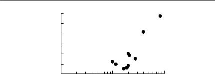
Hudson et al. (1992b) used nine years of data on a grouse population in the north of England to obtain the relationship shown in Fig. 10.7 between mean worm burden and winter mortality. They fitted a linear regression to these data, and estimated α from the gradient. As Hudson et al. (1992b) discuss, this approach could be criticized on the grounds that this relationship is a correlation, rather than a demonstration of cause and effect. A more important issue limiting the application of this approach to other populations is that it could be used only because a long time series was available, in which the mean parasite burden varied over an order of magnitude. Unfortunately, such data are extremely unusual.

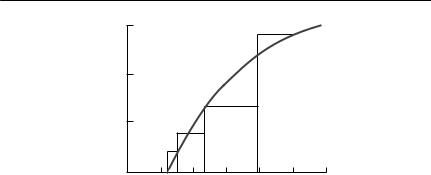
A much more controversial suggestion is that it is possible to infer macroparasite-induced mortality from the distribution of macroparasites within the host population. This idea was first proposed by Crofton (1971). The idea is that mortality amongst the most heavily infected individuals in a

H O S T – P A T H O G E N A N D H O S T – P A R A S I T E M O D E L S 305

negative binomial was a good fit to the distribution of mites on the aquatic insect Sigara ornata, on which they have little effect, but an untruncated distribution was a poor fit to the distribution of mites on Anopheles crucians larvae, on which laboratory experiments indicate that mites have a major effect. Royce and Rossignol (1990) used the method to infer mortality caused by tracheal mites on honey bees. Adjei et al. (1986) fitted a negative binomial to the first few terms of the distribution of a cestode parasite on lizard fish (Saurida spp.), and then extrapolated this to infer a distribution tail that could have been truncated by host mortality.

Effects of infection on host fecundity

Far more attention has been given to estimating parasite and pathogen effects on host survival than on host fecundity. This is somewhat surprising. Models suggest that a pathogen that decreases the fecundity of its hosts may have a greater impact on the host population than one that increases mortality (McCallum & Dobson, 1995). Applying estimates of fecundity from laboratory experiments to wild populations is also more likely to be valid than is applying laboratory estimates of survival to wild populations.

As well as the possibility of outright infertility, the fecundity of infected hosts may be decreased, relative to uninfected hosts, in several ways. There may be a decrease in litter or clutch size, the interval between breeding events may increase, or there may be an increase in the interval between birth and first breeding. Delay in first breeding has a particularly large effect on the intrinsic rate of increase of a population (see Chapter 5), and so parasites that delay the onset of breeding (perhaps by slowing growth) may have a profound effect on the population dynamics of their host. In many ecological models, ‘fecundity’ parameters include early juvenile survivorship (see Chapter 5), so a decrease in juvenile survival because of maternal infection may also be included as a component of parasite impact on fecundity.

A laboratory study by Feore et al. (1997) into the effect of the cowpox virus on the fecundity of bank voles (Clethrionomys glareolus) and wood mice (Apodemus sylvaticus) nicely illustrates some points about disease impact on fecundity. In the UK, cowpox is endemic in these small rodents, but has no demonstrable effect on survival. Feore et al. (1997) dosed pairs of the rodents shortly after weaning, and compared reproductive parameters with control, sham-treated pairs. There were no differences either in the proportion of pairs that reproduced over the 120 days of the experiment, or in the litter size produced. However, infected pairs of both species took significantly longer to produce their first litter than did uninfected pairs. It is interesting that it did not seem to matter whether both parents, or only one parent, was infected. As single-parent infections only occurred when the virus failed to take in one

306 C H A P T E R 1 0

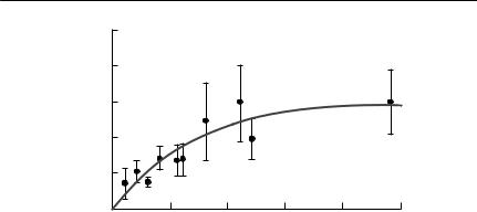
Mean worm intensity (x 103)

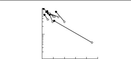
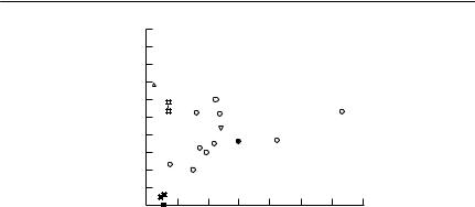
Fig. 10.8 Mean brood size of female grouse as a function of mean worm burden and treatment. The mean brood size (at seven weeks of age) of female grouse treated with anthelminthic (solid circles) is compared with the mean brood size of control females (open circles). Data points from the same year are connected with a line. The mean worm intensity was estimated from shot samples of both treated and control birds. From Hudson et al. (1992b).

parent, the corresponding sample sizes were very small, which would have limited the power of the experiment to detect any difference between dualparent and single-parent infections.

Parasite reduction experiments can also be used to investigate parasite effects on fecundity. For example, Hudson et al. (1992b) treated red grouse females with anthelminthics over a period of eight years. In years of heavy infection, they found significant increases in both mean brood size and hatching success in treated females, compared with controls. The combined data (Fig. 10.8) allowed them to estimate the impact of the parasite on fecundity, as a function of parasite density. It is important to note that the intensity of infection in both treated and control birds could be estimated from birds shot as game.

Parasite parameters within the host

Most simple models of microparasitic infection do not attempt to model explicitly the dynamics of the parasite population within the host. However, it is still necessary to estimate the length of the latent period between a host being infected and becoming infectious, the duration of infection, and the rate at which immunity is lost. Some of these, of course, may be zero. It may also be necessary to estimate an incubation period, which is the time between the infection being acquired and it being detectable. This is not necessarily the same as the latent period. Each of these processes may potentially be quite

H O S T – P A T H O G E N A N D H O S T – P A R A S I T E M O D E L S 307

complex and heterogeneous in some diseases (see Anderson & May, 1991). For example, some individuals may become asymptomatic carriers, which are infectious for a long period, but show few symptoms. The presence of carriers, even if rare, may profoundly alter the dynamics of a disease. In simple cases, however, latent periods, recovery rates, etc. can be estimated by direct observation of infected individuals.

The demographic parameters of parasites within their hosts are far more difficult to deal with in macroparasitic infections. In macroparasites, the rate of adult parasite mortality, parasite fecundity, maturation and growth rates often are all dependent on the intensity of infection in an individual host (Anderson & May, 1991). These density-dependent effects are frequently quite crucial to the overall dynamics of the macroparasite population. As the density dependence occurs within an individual host, its consequences for the population as a whole depend not only on the mean parasite burden, but also on the way in which the parasites are distributed between hosts.

Parasite survival within individual hosts can be measured in experimental situations by recording the decay in parasite infection levels within a host cohort that is no longer exposed to infection. The hosts may either be removed from a natural infective environment, or may be experimentally infected at a single time. Such experiments are rarely carried out in the field, because it is necessary to keep the hosts in an environment in which no further infection occurs. As there is evidence that the survival of parasites may depend strongly on the nutritional status of the host (Michael & Bundy, 1989), extrapolation of laboratory results to field populations should be done with caution. Host immune responses to macroparasites exist, but are poorly understood (Anderson & May, 1991; Grenfell et al., 1995), introducing further complications.

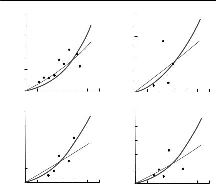
Density-dependent fecundity in macroparasites is often detectable. It is probably the major factor regulating the level of macroparasitic infection (Anderson & May, 1991). Numerous studies have estimated the fecundity of gastrointestinal helminths by recording egg output in faeces as a function of worm burden, determined either by expulsion chemotherapy or by subsequent dissection of the hosts (Anderson & May, 1991; McCallum & Scott, 1994). Some examples of density-dependent fecundity in macroparasites are shown in Fig. 10.9. In general, there is a very high degree of variation in the egg output produced by hosts with a given parasite burden. There are several ways in which density dependence can be quantified. A regression of log(eggs per female worm per day) versus either worm burden itself (Fig. 10.9(a) and (c)) or log(worm burden) (Fig. 10.9(b)) can be used, with negative slope coefficients indicating density dependence. Alternatively, a simple regression of log(egg output) versus log(parasite burden) can be used (Fig. 10.9(e)), and the gradient of the log-log regression can be used to quantify density dependence (a slope less than 1 indicates direct density dependence). Some of the extreme

H O S T – P A T H O G E N A N D H O S T – P A R A S I T E M O D E L S 309

variation in parasite fecundity at a given worm burden may be caused by short-term variation in egg output, but Figs 10.9(c) and (d) show that there is still a lot of variation in fecundity, even if the eggs per female worm can be counted directly.

Basic reproductive number R0 of a parasite

The basic reproductive number is often the critical property of a host–parasite interaction that needs to be measured for predictive purposes. If your objective is to eliminate a pathogen or parasite from a population, the problem is one of reducing R0 to below 1. Conversely, if a pathogen or parasite is contemplated for biological control, a necessary (but not sufficient) condition for success is that R0 > 1. As can be seen for simple models in eqns (10.4) and (10.12), R0 can be defined as a function of more elementary parameters of the host–parasite interaction, together with host density. Similar expressions can be derived for more complex models.

One way to estimate R0 is thus to estimate all the parameters that contribute to R0 in a model appropriate to the particular host–parasite interaction, and then to combine them. This approach has been taken in a number of studies (e.g. Lord et al., 1995). The problem with this approach is not only that many separate parameters must be estimated, but also that each parameter contributing to the final R0 is estimated with uncertainty, and probably is estimated by a different method. Attempting to place some sort of confidence bound around the final estimate is therefore difficult. Woolhouse et al. (1996) addressed this problem by conducting a sensitivity analysis, in which each parameter in turn was varied over its plausible range, and the effect on the estimated R0 was investigated. Sanchez and Blower (1997) used a much more formal sensitivity analysis, with Latin hypercube sampling (see Chapter 2), to assess the uncertainty of an estimate of R0 for tuberculosis in humans. This is the ideal way to approach the problem.

A second way to estimate R0 is to do so directly. This may be possible, provided the system can be assumed to be in equilibrium: the approach is appropriate for endemic but not for epidemic infections. By definition, at equilibrium, R, the actual mean number of secondary cases per current case, is 1. In a microparasitic infection, if the population is homogeneously mixed, the number of secondary cases produced by an infective individual will be proportional to the probability that any contact is with a susceptible individual (Anderson & May, 1991). Thus, R = R0 x, where x is the proportion of susceptible individuals in the population. Hence, at equilibrium.

where x * is the proportion of susceptible individuals in the population at

310 C H A P T E R 1 0

equilibrium. This proportion can often be estimated using serological techniques, providing a quick and approximate estimate of R0. The critical limitation is that the system must be at equilibrium. It is not easy to determine whether this is so, particularly in a wildlife population that may not have been monitored continuously for a long period.

A similar approach can be taken with macroparasites. At equilibrium, in the host population as a whole, each parasite must replace itself with one other parasite in the next generation. Hence,

Here, f is some function describing the joint effect of all the density-dependent factors influencing the parasite population, and M* is the equilibrium mean parasite burden. If all density dependence derives from density dependence in egg output, Anderson and May (1991) show that

where k is the parameter of the negative binomial distribution that inversely describes the degree of aggregation and γ is the exponent in the following relationship between per capita mean parasite fecundity λ(i) and parasite burden i:

Provided estimates of k, M* and γ can be obtained, R0 can then be estimated as

Threshold population density necessary for disease transmission, NT

NT can be calculated from its component parameters, using eqns (10.5) or (10.13), or modified versions for more complex models. As with R0, there are potential problems in combining estimates of a large number of parameters, each estimated with uncertainty. Appropriate sensitivity analysis should always be carried out. In some cases, it may be possible to estimate NT, given an estimate of R0. For example, in the simple, directly transmitted microparasite model described by eqns (10.1)–(10.3),

where NR is the number of animals in the population from which the estimate of R0 was obtained. More generally, R0 is a nonlinear function of population

312 C H A P T E R 1 0

Summary and recommendations

1 The problems of parameter estimation are quite different for microparasites (viruses, bacteria and protozoa) and macroparasites (typically helminths).

2 For macroparasites, several of the key processes are functions of the parasite burden on individual hosts. This means that the way in which the parasites are distributed within the host population is very important.

3 The process of transmission is particularly difficult to parameterize. The relationship between the level of infection and host age is often useful in estimating the rate at which hosts acquire infection in a given environment.

4 There are substantial problems in applying an estimate of a transmission rate obtained in one location to another location, especially if there are major differences in scale or the extent of habitat heterogeneity. In particular, it is difficult to apply estimates of transmission rates obtained in the laboratory to field situations.

5 Parasite or pathogen effects on host death or fecundity are most appropriately estimated in the field. However, it is difficult to do so without manipulative experiments, particularly for endemic infections that do not change substantially in intensity through time. Observational methods based on the truncation of macroparasite frequency distributions cannot be recommended. 6 The basic reproductive number R0 is a key parameter in both microparasite and macroparasite infections. It can be estimated from a combination of more basic parameters, but there are then difficulties in assessing the uncertainty in the resulting estimate. If infections, whether microparasitic or macroparasitic, can be assumed to be at equilibrium, there are simple, approximate ways of estimating R0 directly. R0 is a function of population density.

7 By far the best-understood macroparasite system in wildlife is the red grouse–nematode interaction studied by Hudson, Dobson and colleagues. This study is based on at least 20 years’ work in a species for which large shot samples can be obtained. There are few short-cuts to producing precise parameter estimates for parasite models.