


C H A P T E R 4
Vital statistics: birth, death and growth rates
Introduction |
|
The most elementary equation in population dynamics is |
|
Nt+Δt = Nt + B − D + I − E, |
(4.1) |
where Nt is the population size at some time t, Nt+Δt is the population size some time interval t later, and B, D, I and E are the numbers of births, deaths, immigrants and emigrants in the time period. Having considered problems of estimating population size in the previous chapter, I now move on to the problem of estimating the numbers of births and deaths in a given time interval. Immigration and emigration are considered later, in Chapter 7, on estimating parameters for spatial models.
The estimation problems encountered depend very much on the type of animal under study. In terrestrial vertebrates, the principal problems are likely to be small sample size and lifespans that may exceed that of the study itself. On the positive side, however, it is often possible to follow the fate of particular individuals. In studies of insects and other invertebrates, sample size is not usually a problem, and the lifespan of the study organism is often very short. However, it is frequently impossible to trace particular individuals through time. Fish fall somewhere between these two extremes.
If the parameter estimates are required for a model structured by size or stage, it is essential also to estimate growth and development rates. Fecundity is often related to size, and the mortality through a particular size or stage class depends on how long an individual remains in that class.
Fecundity
There is considerable confusion about the most appropriate definition of fecundity in the ecological literature (Clobert & Lebreton, 1991). The most usual definition is the number of female offspring produced per adult female per unit of time, but there is no consistency on whether ‘females’ means female zygotes, or numbers surviving from the zygote stage to some other lifehistory stage at which the offspring are counted. If the sex ratio is uneven, it will be necessary to include it explicitly to estimate production of males and females separately. Usually, ‘fecundity’ will include some juvenile mortality. The most appropriate definition will depend on the context, and on how
102

V I T A L S T A T I S T I C S : B I R T H , D E A T H A N D G R O W T H R A T E S 103
fecundity is to be used in a model. For example, the particular case of estimating fecundity for the Euler–Lotka equation is discussed in Chapter 5.
In general, fecundity is one of the easier demographic parameters to estimate in birds and mammals. Captive breeding data will usually provide estimates of gestation period and clutch or litter size that can be applied to wild populations without too much error. One adjustment that does need to be made, however, is to estimate the proportion of adult females that are breeding in a given population at a particular time. This is not a straightforward exercise (see Clobert et al., 1994). In the fisheries literature, much attention is given to estimating fecundity, usually by estimating the number of eggs carried by gravid females. This is valuable for determining the relative contribution of various age or size classes to the overall reproductive output of the population. Without an estimate of larval mortality, however, it sheds limited light on the reproductive output itself.
Fecundity will always be age-dependent. It is frequently also sizedependent, particularly in ectothermic animals. Juveniles, by definition, do not reproduce, and in almost all organisms the pre-reproductive stage is not such a small fraction of the total lifespan that it can be neglected. This is especially so because the intrinsic growth rate of a population is particularly sensitive to early reproduction (see Chapter 5). Nevertheless, some very abstract models (for example, the simple host–parasite models of Anderson and May, 1978) assume a single birth-rate parameter and require it to be separated from the death rate. Attempting to estimate this as simply the rate of production of offspring by mature females will always cause a gross overestimate of the intrinsic growth rate of the population, to an extent that the qualitative behaviour of the system will probably be misrepresented.
There is no entirely satisfactory way to replace an age-specific fecundity estimate with a simple, unstructured rate. Probably the best approach is to use the full age-specific fecundity and mortality schedules to estimate the intrinsic rate of growth r (see Chapter 5), and then to subtract the death rate from this to yield a single birth-rate parameter.
Survival
Survival is inevitably a much more difficult process to quantify in wild populations than is fecundity. Survival of captive animals will always be a very poor indicator of survival in the wild, except that it may give an indication of the absolute maximum age the animals can reach. Estimating the rate of survival in the field ideally involves following the fate of individuals, preferably of known age. Given restrictive assumptions, some idea of the age-specific death rate can be gained from the age distribution of animals, but this requires a means of ageing individuals, a problem that is often technically difficult.

104 C H A P T E R 4
The most appropriate ways to describe survival for a model and then to estimate parameters to quantify the chosen form of survival depend critically on the type of organism under study and on the objectives of the study. In any but the most general models, the death rate will be a function of age. The death rate at a given age may also be dependent on time and any number of other variables.
Broadly speaking, the pattern of age-dependent survival in a population can be described in two ways. A life table breaks the life history up into a number of discrete ages or stages, and estimates a survival rate through each stage. A survival curve represents the death rate as a function of age. From the perspective of parameter estimation, the difference between the two approaches is similar to the difference between analysis of variance and regression. A life table requires the estimation of as many survival rates as there are stages in the table, but is completely flexible in the way that it allows survival to change with age. A survival curve will generally require the estimation of two or three parameters only, depending on the functional form fitted, but the way in which survival changes with age is constrained. Alternatively, a life table can be viewed as expressing survival as a nonparametric function of age, in contrast to the parametric approach of a survival curve (Cox & Oakes, 1984, p. 48).
Studies of insects generally have few problems with sample size, and often use life-table approaches to advantage. In many studies of vertebrate populations, however, sample size is a major constraint, and estimating many parameters simultaneously is impractical. An approach based on a twoor three-parameter survival curve may thus be preferable to a life table, even if the resulting mortality estimates are subsequently used in a model with discrete age classes.
Particular problems arise with models that are structured by size or developmental stage. For a given death rate per unit of time, the proportion of individuals surviving through a life-history stage will obviously depend on the time spent in that stage. Unless the development time through a stage is fixed, parameterization of stage-specific survival requires simultaneous estimation of the development and mortality rates.
The most appropriate method of estimating survival also depends on a number of practical considerations. Some methods can only be used if animals can be individually marked and then followed reliably until either death or the end of the study. If individuals are marked, but will not necessarily be detected on every sampling occasion, even if alive and in the study area, then other methods must be used. It may be possible to mark or identify members of, or a sample from, a cohort, but not to follow particular individuals through time. Again, different estimation methods must be used. Finally, in many situations, it is not possible to mark animals in any way, and attempts must be made to estimate survival from the age or size distribution of the animals.

V I T A L S T A T I S T I C S : B I R T H , D E A T H A N D G R O W T H R A T E S 105
Faced with this diversity of problems and possible approaches, I will first develop some general principles and concepts, and then deal with the actual estimation problems in a series of subsequent sections. Table 4.1 provides a guide to the possible approaches that can be taken to estimate survival or mortality rates.
Survival curves, failure times and hazard functions
A survival curve or survivor function is simply the proportion of individuals surviving as a function of age or time from commencement of the study. In the general ecological literature, it has become conventional to divide survival curves into three types, I, II and III (Krebs, 1985; Begon et al., 1996a) (Fig. 4.1), depending on whether the relationship between log survivors and age is concave, straight or convex. These types correspond to death rates that are decreasing, constant or increasing with age. Almost all survival curves for real organisms, however, will include segments with very different survival rates, corresponding to different ontogenetic stages.
It is tempting to estimate a survivor function by fitting a line or curve through a plot of the proportion of individuals surviving versus time. This approach is invalid statistically because successive error terms are not independent: the survivors at any time have also survived to each previous time step. A better approach is to use the time until death of each individual (its ‘failure time’ in the statistical literature) as the response variable. A problem which then arises is that it is likely that some individuals will either survive to the end of the study or otherwise be removed. A minimum failure time can be assigned to these individuals, but the actual failure time is unknown. Such observations are ‘censored’.
Survival of individuals throughout the course of a study is the most obvious way that censoring can occur, and will result in observations censored at a value equal to the total study duration. Censoring may, however, occur at other values. In many studies, subjects may enter the study at different times. For example, animals may be caught and radio-collared at times other than the start of the study. This is known as ‘staggered entry’ (Pollock et al., 1989), and individuals surviving at the conclusion of the study period will have different censoring times, depending on their time of entry (Fig. 4.2). Alternatively, individuals may be removed from the study before its conclusion, due to factors other than natural mortality. Possibilities include trap mortality, permanent emigration, or radio-collar failure.
Statisticians usually describe survival data in terms of the hazard function, or the probability density of death as a function of time, conditional on survival to that time (Cox & Oakes, 1984). To ecologists, this concept will be more familiar as the instantaneous death rate of individuals, as a function

Table 4.1 A key for choosing a method of survival analysis. Use this like a standard dichotomous key for identifying organisms. Start at 1, on the left-hand side, and decide which of the alternatives best applies to your problem. Then go to the number associated with that alternative, and repeat the process. Continue until you reach a suggested method, or you reach a 5, which indicates that there is no satisfactory method
1Do you want a continuous survival function or a life table (survival in discrete stages or intervals)?
Survival function |
2 |
Life table |
7 |
2Can particular individuals be followed through time?
Yes 3
No 6
3Can all individuals being followed in the population be detected at each sampling occasion, if they are present, or may some be missed?
|
All detected if present |
4 |
|
Some may be missed |
5 |
4 |
Parametric survival analysis (see p. 108) |
|
5 |
Mark–resight and mark–recapture methods (see p. 119) |
|
6Can the number of survivors from an initial cohort of known size be determined?
Yes 4
No 5
7Can you follow an initial cohort through time?
Yes 8
No 13
8Are the intervals of the life table of fixed (but not necessarily equal) duration, and can individuals be assigned to an interval unequivocally?
Yes 9
No 12
9Do you need to use statistical inference, or is simple description sufficient?
|
Description only |
10 |
|
Statistical inference required |
11 |
10 |
Cohort life-table analysis (see p. 116) |
|
11 |
Kaplan–Meier method (see p. 118) |
|
12 |
Stage–frequency analysis (see p. 126) |
|
13 |
Can individuals be aged? |
|
|
Yes |
14 |
|
No |
18 |
14 |
Can the proportions of each age class surviving one time step be determined? |
|
|
Yes |
15 |
|
No |
16 |
15 |
Standard life-table techniques possible, but yields a current or |
|
|
time-specific life table (see p. 116) |
|
16 |
Is the rate of population increase known (or can it be assumed to be 0)? |
|
|
Yes |
17 |
|
No |
5 |
17 |
Use ‘methods of last resort’ (see p. 130) |
|
18 |
Try stage–frequency analysis (see p. 126) |
|
|
|
|
Proportion surviving
(a)
1.0
0.8
0.6
0.4
0.2
0.0
V I T A L S T A T I S T I C S : B I R T H , D E A T H A N D G R O W T H R A T E S 107
|
1.000 |
surviving |
0.100 |
Proportion |
0.010 |
|
|
|
0.001 |
0 |
50 |
100 |
150 |
200 |
0 |
50 |
100 |
150 |
200 |
|
Age (arbitrary units) |
|
|
(b) |
Age (arbitrary units) |
|
|
||
|
|
|
|
|
|
|
|
|
|
Fig. 4.1 Survival curves of types I, II, and III, with survival: (a) on a linear scale; (b) on a log scale. The solid line is a type I survival curve, the dotted line is a type II curve, and the dashed line is a type III curve. These were generated using a Weibull survival function (see
Table 4.3), with: κ = 5 and ρ = 0.007 36 (type I), κ = 1 and ρ = 0.034 54 (type II); and κ = 0.2 and ρ = 78.642 (type III). I chose values of ρ so that survival to age 200 was standardized at 0.001 for each value of κ.
Animal
5
4
3
2
1
0 |
1 |
2 |
3 |
4 |
5 |
Time units
Fig. 4.2 Staggered entry and censoring in a survival study. This diagram represents the fates of five individuals in a hypothetical survival experiment running from times 0 to 5. The horizontal lines represent times over which animals were part of the study. Deaths are marked by solid dots, and open dots indicate right-censored observations: it is known that the animal survived to at least the time shown, but its actual time of death is unknown. Animal 1 was followed from the beginning of the study, and survived through to the end, so its survival time is right-censored at 5 time units. Animal 2 similarly was followed from the beginning, but was dead at time 4. Animal 3 did not enter the study until time 1, and was dead at time 4. Animal 4 entered the study at time 2, but at time 4 its radio-collar had failed, so it was not known if it was alive or dead. Its survival time is therefore censored at 2 time units. Finally, animal 5 entered the study at time 3, and survived until the end. Its survival time is thus also censored at 2 time units.
108 |
C H A P T E R 4 |
|
|
|
|
|
|
Table 4.2 Ways of representing the probability of survival |
|
|
|
|
|
||
|
|
|
|
|
|
||
|
|
|
Relationship to other |
||||
Function Name |
Meaning |
representations |
|
||||
|
|
|
|
|
|
|
|
S(t) |
Survivorship function |
Proportion of cohort surviving |
|
|
|
t |
|
|
|
to time t |
|
|
|
|
|
|
|
|
S(t) = exp |
− μ(u)du |
|||
|
|
|
|
|
|
|
|
|
|
|
|
|
0 |
|
|
μ(t) |
Age-specific death rate, |
Probability density of failure at |
μ(t) = f(t)/S(t) |
|
|||
|
or hazard function |
time t, conditional on survival |
|
|
|
|
|
|
|
to time t |
|
|
|
|
|
f (t) |
|
Probability density of failure at |
f (t) = − |
dS(t) |
|
|
|
|
|
time t |
|
dt |
|
|
|
|
|
|
|
|
|
|
|
of age. Survival can also be described as an unconditional probability density of failure as a function of age. This is different from an age-specific death rate, because it is the probability density of death at a given age of an individual at the start of the study. The unconditional probability density of failure is important, as it is this quantity that is necessary for maximum likelihood estimation of survival rate parameters. Table 4.2 summarizes these ways of describing age-specific survival, and the relationships between them.
Parametric survival analysis
The approaches described in this section produce an estimate of survival as a continuous function of age or time from the entry of the subject into the study. Survival may also depend on other variables, either continuous or categorical. These approaches can be applied in two situations: if animals are marked individually, and their continued survival at each sampling occasion can be determined unequivocally; or if animals are not followed individually, but the numbers from an initial cohort surviving to each sampling occasion can be counted. If animals are marked individually, but may not necessarily be detected on each sampling occasion, the mark–recapture methods discussed later in the chapter should be used instead.
It is first necessary to select an explicit functional form for the hazard function (the death rate, as a function of age), and the objective is then to estimate the parameters of that function. There are many forms of the hazard function in the statistical literature (see Cox & Oakes, 1984, p. 17). For most ecological purposes, two are adequate: a constant hazard or death rate, which yields an exponential survival function; and the Weibull distribution, which allows the hazard to either increase or decrease with time depending on the value of an adjustable parameter. Table 4.3 gives the hazard, probability density and

V I T A L S T A T I S T I C S : B I R T H , D E A T H A N D G R O W T H R A T E S 109
Table 4.3 Exponential and Weibull survival curves
Name |
Hazard function |
Density function |
Survivorship function |
|
|
|
|
Exponential |
ρ |
ρe−ρt |
e−ρt |
Weibull |
κρ(ρt)κ−1 |
κρ(ρt)κ−1 exp[−(ρt)κ ] |
exp[−(ρt)κ ] |
survival functions of these two models. The exponential distribution has a single parameter ρ, which is the instantaneous death rate per unit of time. The Weibull distribution also has a rate parameter ρ, and, in addition, a dimensionless parameter κ, which determines whether the hazard increases or decreases with time. From Table 4.3, it can be seen that κ > 1 generates a death rate increasing with time (a type III survival curve) and that if κ < 1, the death rate decreases with time (a type I curve). If κ = 1, the Weibull reduces to the exponential distribution. Figure 4.1 shows examples of Weibull and exponential survival functions.
In many cases, it may be necessary to describe survival as a function of explanatory variables. These might be continuous, such as parasite burden, or discrete, such as sex. It is relatively straightforward to make ρ a function of such explanatory variables. For example, if a continuous variable X affects survival, ρ can be represented as
ρ(X ) = exp(α + βX ), |
(4.2) |
where α and β are parameters to be estimated. The exponential ensures that the death rate remains positive for all values of α, β and X. It is usual to assume that the index κ remains constant and does not depend on the value of the explanatory variable, although there is no good biological, as distinct from mathematical, reason why this should be so.
Most ecologists will use a statistical package to fit a survival function, although it is not difficult to do using a spreadsheet from the basic principles of maximum likelihood. Some statistical packages (for example, SAS) use a rather different parameterization from the one I have described here, which follows Cox and Oakes (1984). It is important to plot out the observed and predicted survival, both to assess the fit of the model visually, and to ensure that the parameter estimates have been interpreted correctly.
The survival rate of black mollie fish infected with Ichthyophthirius multifiliis (Table 4.4), an example first discussed in Chapter 2, is modelled using the Weibull distribution in Box 4.1, with the results presented graphically in Fig. 4.3. It is clear from the figure that the Weibull curve, using parasite burden as a continuous linear covariate, does not completely capture all the differences in survival between the different levels of parasite infection. In particular, the predicted mortality rate is too high for the lowest infection

110 C H A P T E R 4
class. The fit can be improved by estimating a separate ρ for each infection class. This example emphasizes that procedures such as checking for linearity and lack of fit, which are standard practice for linear models, are equally important for survival analysis.
If very few data are available, the simplest and crudest way to estimate a death rate is as the inverse of life expectancy. If the death rate μ is constant through time, then the following differential equation will describe N(t), the number of survivors at time t:
|
dN |
= −μN(t). |
(4.3) |
|
|
||
|
dt |
|
|
This has a solution |
|
||
N(t) = N(0) exp(−μt). |
(4.4) |
||
Table 4.4 Black mollie survival data. The following table shows, as a function of parasite burden, the number of fish N that had died at the given times (in days) after the initial assessment of infection. The experiment was terminated at day 8, so that it is not known when fish alive on that day would have died. The survival time of those fish is thus censored at day 8
Burden |
fail time |
N |
Burden |
fail time |
N |
|
|
|
|
|
|
10 |
6 |
1 |
90 |
4 |
1 |
10 |
8* |
10 |
90 |
5 |
2 |
30 |
3 |
1 |
90 |
6 |
1 |
30 |
7 |
2 |
90 |
7 |
1 |
30 |
8 |
4 |
90 |
8* |
2 |
30 |
8* |
3 |
125 |
3 |
1 |
50 |
3 |
2 |
125 |
4 |
4 |
50 |
4 |
1 |
125 |
5 |
1 |
50 |
5 |
3 |
125 |
6 |
2 |
50 |
6 |
1 |
125 |
8 |
1 |
50 |
7 |
3 |
175 |
2 |
2 |
50 |
8 |
5 |
175 |
3 |
4 |
50 |
8* |
3 |
175 |
4 |
3 |
70 |
4 |
2 |
175 |
5 |
3 |
70 |
5 |
2 |
175 |
8 |
1 |
70 |
6 |
1 |
225 |
2 |
4 |
70 |
7 |
1 |
225 |
3 |
4 |
70 |
8 |
4 |
225 |
8 |
1 |
70 |
8* |
4 |
300 |
2 |
1 |
|
|
|
300 |
3 |
1 |
|
|
|
300 |
4 |
4 |
|
|
|
300 |
6 |
2 |
|
|
|
300 |
7 |
1 |
|
|
|
|
|
|
*Censored observations.

V I T A L S T A T I S T I C S : B I R T H , D E A T H A N D G R O W T H R A T E S 111
Box 4.1 Fitting a Weibull survival function using maximum likelihood
The data used in this example are from an experiment investigating the survival of black mollie fish infected by the protozoan Ichthyophthirius. The experimental procedure is outlined in the legend to Table 2.1, and the data are presented in Table 4.4. The time of death of individual fish, up to a maximum of eight days after assessment of the infection level (which in turn was two days after infection) was recorded as a function of intensity of parasite infection. The objective is to use maximum likelihood to fit a Weibull survival curve with parasite infection intensity X as a covariate, and the rate parameter of the Weibull distribution given by
ρ = exp(α + βX ). |
(1) |
There are two types of observation in the data set: uncensored observations, for which the actual time until death is known; and censored observations, for which it is known that the fish survived at least eight days, but the actual time of death is unknown. The probability density of death at time t, where t ≤ 8, is given in Table 4.3:
f(t) = κρ(ρt)κ−1 exp[−(ρt)κ ]. |
(2) |
The probability that a fish survives beyond eight days is given by the survivorship function, evaluated at t = 8:
S(8) = exp[−(8ρ)κ ]. |
(3) |
The log-likelihood function has two components, one for uncensored observations, and a second for the censored observations. Following the usual approach of maximum likelihood estimation, the log-likelihood function of the three unknown parameters α, β and κ can then be written as a function of the observed data:
|
|
|
|
l(α,β,κ ) = ∑ln( f (t)) + ∑ln(S(t)). |
(4) |
||
|
u |
c |
|
Here, the u represents a sum over the uncensored observations, and the c a sum over the censored observations. (Note that in this case, the time at censoring entered into S(t) is 8 for every censored observation.) The maximum likelihood estimates of the parameters are those which maximize the value of eqn (4). Most ecologists would probably use a statistical package to perform the calculation. It is, however, quite straightforward to do using a spreadsheet. Substituting eqns (2) and (3) into eqn (4), the problem is to maximize
|
|
|
l(ρ,κ ) = ∑(ln κ + κ ln ρ + (κ − 1)ln(t) − (ρt)κ ) − ∑(ρt)κ . |
(5) |
|
u |
c |
|
|
|
|
continued on p. 112

112 C H A P T E R 4
Box 4.1 contd
Substituting the expression for ρ from eqn (1), and further simplifying, the objective is to find estimates of α, β and κ to maximize
|
|
|
l(α ,β,κ ) = ∑[ln κ + κ(α + βX) + (κ − 1)ln(t)]− ∑(t exp(α +βX))κ . |
(6) |
|
u |
u,c |
|
|
|
|
This can be done using the Solver facility in Excel, as is shown for a simpler example in Box 2.3. In this case, all that is necessary is to enter each component of the sums in eqn (6) into separate rows of a spreadsheet, and to maximize their sum. The solutions are:
α |
β |
κ |
|
|
|
−2.211 56 |
0.002 789 |
2.892 263 |
|
|
|
As would be expected, β is positive, meaning that the death rate increases with parasite burden. As κ > 1, the death rate for a given parasite burden also increases strongly with time since infection. This is also to be expected, given that this is a parasite which grows rapidly in size over its 10-day lifetime on the host.
The predicted survival curves are shown in Fig. 4.3. Whilst the fit seems fairly good for intermediate parasite burdens, there is evidence of systematic differences between observed and predicted survivals, particularly at the lowest infection intensity. This subjective impression is confirmed if separate values of ρ are fitted for each value of the parasite burden. Again, this can be done quite easily on a spreadsheet. The estimated parameters are shown below.
Burden |
10 |
30 |
50 |
70 |
90 |
125 |
175 |
225 |
300 |
|
|
|
|
|
|
|
|
|
|
ln(ρ) |
−2.860 88 |
−2.139 94 |
−1.987 8 |
−2.073 74 |
−1.979 54 |
−1.670 69 |
−1.509 17 |
−1.427 54 |
−1.59 146 |
|
|
|
|
|
|
|
|
|
|
The estimated value of κ is 3.00.
The change in deviance (twice the difference in the log-likelihood between the two models) is 23.58 at a cost of 7 additional parameters, a highly significant difference. The predicted survival using this categorical model is also shown in Fig. 4.3.
V I T A L S T A T I S T I C S : B I R T H , D E A T H A N D G R O W T H R A T E S 113
Burden=10
|
1.0 |
|
|
|
|
|
surviving |
0.8 |
|
|
|
|
|
0.6 |
|
|
|
|
|
|
Proportion |
|
|
|
|
|
|
0.4 |
|
|
|
|
|
|
|
|
|
|
|
|
|
|
0.2 |
|
|
|
|
|
|
0.00 |
2 |
4 |
6 |
8 |
10 |
(a) |
|
|
|
|
|
|
|
1.0 |
|
|
|
|
surviving |
0.8 |
|
|
||
0.6 |
|
|
Proportion |
|
|
0.4 |
|
|
|
|
|
|
0.2 |
|
|
|
|
|
0.00 |
|
(b) |
||
|
1.0 |
|
|
|
|
surviving |
0.8 |
|
|
||
0.6 |
|
|
Proportion |
|
|
0.4 |
|
|
|
|
|
|
0.2 |
|
|
|
|
(c) |
0.00 |
|
|
|
|
Burden=30
2 |
4 |
6 |
8 |
10 |
Burden=50
2 |
4 |
6 |
8 |
10 |
|
Time since infection (days) |
|
|
|
Fig. 4.3 Survival of black mollies infected with Ichthyophthirius multifiliis. Black dots show the observed proportions of fish surviving as a function of time after infection. The proportion surviving as predicted by a Weibull survival function, using burden as a continuous linear predictor, is shown as a solid line. The dotted line and open circles
show the predicted proportion surviving if a Weibull with burden treated as a categorical variable is used.
114 C H A P T E R 4
|
1.0 |
|
|
|
|
surviving |
0.8 |
|
|
||
0.6 |
|
|
Proportion |
|
|
0.4 |
|
|
|
|
|
|
0.2 |
|
|
|
|
|
0.00 |
|
(d) |
||
|
1.0 |
|
surviving |
0.8 |
|
|
||
0.6 |
|
|
Proportion |
|
|
0.4 |
|
|
|
|
|
|
0.2 |
|
|
|
|
|
0.0 |
|
|
|
|
|
0 |
|
(e) |
||
|
1.0 |
|
|
|
|
surviving |
0.8 |
|
|
||
0.6 |
|
|
Proportion |
|
|
0.4 |
|
|
|
|
|
|
0.2 |
|
|
|
|
|
0.00 |
|
(f) |
||
Burden=70
2 |
4 |
6 |
8 |
10 |
Burden=90
2 |
4 |
6 |
8 |
10 |
|
|
|
Burden=125 |
|
2 |
4 |
6 |
8 |
10 |
|
Time since infection (days) |
|
|
|
Fig. 4.3 contd

V I T A L S T A T I S T I C S : B I R T H , D E A T H A N D G R O W T H R A T E S 115
|
1.0 |
|
|
|
|
surviving |
0.8 |
|
|
||
0.6 |
|
|
Proportion |
|
|
0.4 |
|
|
|
|
|
|
0.2 |
|
|
|
|
|
0.00 |
|
(g) |
||
|
1.0 |
|
surviving |
0.8 |
|
|
||
0.6 |
|
|
Proportion |
|
|
0.4 |
|
|
|
|
|
|
0.2 |
|
|
|
|
|
0.0 |
|
|
|
|
|
0 |
|
(h) |
||
|
1.0 |
|
surviving |
0.8 |
|
|
||
0.6 |
|
|
Proportion |
|
|
0.4 |
|
|
|
|
|
|
0.2 |
|
|
|
|
|
0.0 |
|
|
|
|
|
0 |
|
(i) |
|
|
Burden=175
2 |
4 |
6 |
8 |
10 |
Burden=225
2 |
4 |
6 |
8 |
10 |
|
|
|
Burden=300 |
|
2 |
4 |
6 |
8 |
10 |
|
Time since infection (days) |
|
|
|
Fig. 4.3 contd

116 C H A P T E R 4
The definition of life expectancy, E(t), is the average age each individual survives from time 0, and hence
∞
t exp(−μt)dt
E(t) = |
t =0 |
. |
(4.5) |
|
|||
∞ |
|||
|
exp(−μt)dt |
|
|
t =0
Integrating by parts, the solution to this is simply 1/μ.
This straightforward relationship is useful where a single death-rate parameter needs to be plugged into a model, as long as you remember that the life expectancy of an organism or life-history stage is usually much shorter than the maximum lifespan.
Life tables
A life table is simply a record showing the number of survivors remaining in successive age classes, together with a number of additional statistics derived from these basic data (Table 4.5). The method has its basis in human demography, and in particular, the life insurance industry (see Keyfitz, 1977). It is the first stage in constructing many ageor stage-structured models. The simplest life tables are single-decrement life tables, in which individuals dying in each age class or stage are recorded, without any attempt to identify the cause of death. A multiple-decrement life table (Carey, 1989) seeks further to attribute deaths to a range of possible causes, permitting the impact of various mortality factors on the population to be determined.
In developed countries, a full register of births and deaths for many years makes obtaining the data for human populations a straightforward exercise. Many animal and plant populations are a very different matter. With long-lived organisms, in particular, it is usually impossible to follow an entire cohort from birth to death. A wide variety of methods has been developed to deal, as far as is possible, with problems of limited sample size, limited study duration, organisms with unknown fate, difficulties with ageing and other sampling difficulties.
There are two basic forms of life table, whether singleor multipledecrement tables are considered. The standard form is the cohort life table, in which a number of organisms, born at the same time, are followed from birth, through specified stage or age classes, until the last individual dies. The ageor stage-specific survival rates obtained are therefore for a number of different times, as the cohort ages. The second form of life table, a current life table, takes a snapshot of the population at a particular time, and then determines the survival over one time period for each age or stage class in the population.

V I T A L S T A T I S T I C S : B I R T H , D E A T H A N D G R O W T H R A T E S 117
Table 4.5 Structure of a basic single decrement life table. The simplest life table is a complete cohort life table, which follows an initial cohort of animals from birth until the death of
the last individual. Two fundamental columns only are required to calculate the table, the age class (conventionally represented as x) and the number of individuals alive at the commencement of the age class (conventionally represented as Kx). From these, a further
seven columns can be derived. Note that a life table sensu stricto is concerned with mortality only. Age-specific fertility is often added, and is of course essential for answering ecological questions about population growth rate, reproductive value and fitness. After Carey (1993)
Column |
Definition |
Calculation |
|
|
|
x |
Age at which interval begins, relative to initial cohort |
Basic input |
Kx |
Number alive at the beginning of age class x |
Basic input |
Dx |
Number dying in interval x to x + 1 |
Dx = Kx+1 − Kx |
lx |
Fraction of initial cohort alive at beginning of interval x |
lx = Kx /K0 |
px |
Proportion of individuals alive at age x that survive |
px = lx+1/lx |
|
until age x + 1 |
|
qx |
Proportion of those individuals alive at age x that |
qx = 1 − px |
|
die in the interval x to x + 1 |
|
dx |
Fraction of the original cohort that dies in |
|
the interval x to x + 1 |
Lx |
Per capita fraction of age interval lived in the |
|
interval from x to x + 1 |
Tx |
Total number of time intervals lived beyond age x |
ex |
Further expectation of life at age x |
dx = lx − lx+1 or dx = Dx /K0
Lx |
= lx |
− |
dx |
|
2 |
||||
|
|
|
∞
Tx = ∑Lz
z =x
ex = Tx /lx
An abridged life table is simply one that has been amalgamated into a number of life-history stages, not necessarily of equal length. In the ecological literature, it would more often be called a stage-structured life table. The components of such a table are identical to the complete table, with the exception that Lx needs to be adjusted to take account of the varying length of each interval. Hence
|
|
|
|
|
d |
x |
|
L |
x |
= n l |
x |
− |
|
, |
|
|
|
||||||
|
|
|
2 |
||||
where n is the duration in time units of the life-history stage from x to x + 1. The idea here is simply that a proportion lx of the individuals present initially enter the life-history stage, and those that die in the interval (a fraction dx of the initial cohort) survive, on average, half the interval.
Fairly obviously, both methods will only be equivalent if death rates remain constant through time.
Cohort life tables
The simplest way conceptually of obtaining a life table is to identify or mark a
118 C H A P T E R 4
large number of individuals at birth, and then to follow those individuals until the last individual dies. This approach is straightforward for univoltine insects, in which all of a single cohort is present at any given time, and the number of individuals followed can be very large indeed. There is a massive literature on the use of such life tables in applied entomology (see Carey, 1993, for a review). In many such cases, the life table is a set of descriptive statistics for the particular cohort under examination, so that estimation problems and determination of standard errors, etc. are not relevant. In other circumstances, particularly in studies of vertebrate populations, a sample of individuals in a single cohort may be identified and these may be intended to act as a basis for making inferences about the entire cohort. If this is the objective, statistical inference is involved. This can be done using the Kaplan–Meier or productmoment estimator (Cox & Oakes, 1984, p. 48).
Kaplan–Meier method
The idea behind this approach is simply that the Kx individuals entering age class x can be considered as independent binomial trials, and that the objective is to estimate the probability of failure in the stage. Using the notation of Table 4.5,
+x = Dx .
K x
From this, it is easy to calculate an estimated survivorship function,
|
|
D |
|
:(x) = ∏ 1 |
− |
j |
. |
|
|||
j<x |
|
K j |
|
(4.6)
(4.7)
Equation (4.7) simply states that the proportion of individuals surviving from birth through to a given life-history stage can be obtained by multiplying the proportions that survive through each previous life-history stage. If there are no censored observations, eqn (4.7) will be exactly the same thing as lx in the standard life table notation of Table 4.5. However, if observations are censored before the end of the study, the standard life-table formulation cannot be used. If Kx is considered to be the number of individuals at risk at time x (so that any censoring is assumed to act exactly at x, as would be the case if censoring occurred through trap mortality), then eqn (4.7) permits the survivorship to be estimated.
Approximate confidence intervals for the survivorship function can be calculated using Greenwood’s formula (Cox & Oakes, 1984, p. 51),
var[:(x)] = [:(x)]2 ∑ |
Dj |
. |
(4.8) |
|
|||
j < x |
K j (K j − Dj ) |
|
|

V I T A L S T A T I S T I C S : B I R T H , D E A T H A N D G R O W T H R A T E S 119
This can be used to generate a confidence limit using the normal approximation. A more elaborate, but more accurate approach, particularly for the tails of the distribution, is to use profile likelihood-based confidence intervals (see Chapter 2; and Cox & Oakes, 1984, p. 51).
Whichever approach is used, any method based on binomial survivorship rests on the assumption that the probability of survival for each individual is independent. This will not be the case in many real situations. For example, one might expect heterogeneity in insect survival at a variety of scales, from individual plants through fields to regions. The use of standard binomial theory to calculate survival in such cases will result in the underestimation of confidence bounds, and such underestimation may be gross. The only solution is to measure survival rates separately for each subpopulation and to use the observed variation as a basis for estimation of the standard error in survival across subpopulations.
For many populations, following a set of individuals from birth is impractical. If detecting survivors relies on trapping to resighting, some animals may be missed on each sampling occasion, and may even never be recorded again, although they continue to live in the population. If cohorts overlap, it is necessary to mark and follow particular individuals to apply the standard approach, but this is often impossible. Other species may be so long-lived that no study of reasonable duration can follow a single cohort. A variety of less direct approaches must therefore be used.
Mark–resight and mark–recapture methods
I discussed methods for estimating population size using mark–recapture and mark–resight data in Chapter 3, and mentioned the fact that open-population methods also allow the estimation of recruitment and survival rates. In general, mark–resight or mark–recapture methods are rather more robust at estimating survival rates than population size. Most methods for estimating population size from mark–recapture data depend critically on the basic assumption that, on a given sampling occasion, the capture probability of all individuals is identical. This assumption is not as important for estimating survival rates. It is merely necessary that the survival rate of marked and unmarked animals should be the same, because the survival estimates are based on marked animals only. Reviews of the use of mark–resight and mark–recapture methods for estimating survival are provided by Lebreton et al. (1992) and Cooch and White (1998). The basic idea behind these approaches is discussed in Chapter 3, and follows theory first developed by Cormack (1964).
Mark–recapture methods for estimating survival require estimation of two sets of parameters: capture probabilities and survival probabilities. These parameters may depend on both the time at which an animal is recaptured,

120 C H A P T E R 4
Table 4.6 Parameters in an open mark–recapture study for a standard Cormack–Jolly–Seber model with six capture occasions. (a) Survival probabilities φ: the survival probability φt is the probability of survival from time t until time t + 1
|
Capture time t |
|
|
|
|
|
Time of first |
|
|
|
|
|
|
|
|
|
|
|
|
|
capture (cohort) i |
1 |
2 |
3 |
4 |
5 |
6 |
|
|
|
|
|
|
|
1 |
φ1 |
φ2 |
φ3 |
φ4 |
|
φ5 |
2 |
|
φ2 |
φ3 |
φ4 |
|
φ5 |
3 |
|
|
φ3 |
φ4 |
|
φ5 |
4 |
|
|
|
φ4 |
|
φ5 |
5 |
|
|
|
|
|
φ5 |
Table 4.6 continued. (b) Capture probabilities: the capture probability pt is the probability that a marked animal, which is present in the population at time t, will be caught at that time. The final p6 and φ5 cannot separately be estimated, although their product p6φ5 can be. Modified from Lebreton et al. (1992) and Cooch and White (1998)
|
Capture time t |
|
|
|
|
|
Time of first |
|
|
|
|
|
|
|
|
|
|
|
|
|
capture (cohort) i |
1 |
2 |
3 |
4 |
5 |
6 |
|
|
|
|
|
|
|
1 |
|
p2 |
p3 |
p4 |
p5 |
p6 |
2 |
|
|
p3 |
p4 |
p5 |
p6 |
3 |
|
|
|
p4 |
p5 |
p6 |
4 |
|
|
|
|
p5 |
p6 |
5 |
|
|
|
|
|
|
|
|
|
|
|
|
|
and on the time at which it was first captured. The recapture probabilities pit give the probability of an animal, which was first captured at time i, being recaptured at time t. The survival probabilities φit give the probability of an animal, which was first captured at time i, surviving over the period from t to t + 1. As with the Jolly–Seber method, discussed in Chapter 3, it is not possible, in general, to distinguish marked animals that did not survive the last recapture interval from those that survived, but were not captured at the final capture time. In the most general case, there will be (k − 1)2 separate parameters that can be estimated if there are k capture occasions. Usually, however, a model simpler than the full one can be used.
The Cormack–Jolly–Seber model, first discussed in Chapter 3, has the parameter structure shown in Table 4.6. Survival and recapture probabilities vary between sampling times, but do not depend on when the animal was first caught. Often, a still simpler model with fewer parameters will be adequate. Recapture probabilities or survivals may be constant through time, or it may be possible to predict survival using a logistic regression with a covariate such as rainfall. If this can be done, survival over any number of periods can be modelled with two parameters only.

V I T A L S T A T I S T I C S : B I R T H , D E A T H A N D G R O W T H R A T E S 121
Table 4.7 Survival probabilities for an age-structured model. This matrix of survival probabilities is for a model in which there are three age classes – juveniles, subadults and adults – and six capture times. At first capture, all animals caught are juveniles. If they have survived one capture interval, they become subadults, and if they survive two capture intervals, they become adults. Survival depends only on age, and not time. The probability of survival through the juvenile stage is φj, the probability of survival through the subadult stage is φs, and the survival through each sampling period for adults is φa
|
Capture time t |
|
|
|
|
|
Time of first |
|
|
|
|
|
|
|
|
|
|
|
|
|
capture (cohort) i |
1 |
2 |
3 |
4 |
5 |
6 |
|
|
|
|
|
|
|
1 |
φj |
φs |
φa |
φa |
|
φa |
2 |
|
φj |
φs |
φa |
|
φa |
3 |
|
|
φj |
φs |
|
φa |
4 |
|
|
|
φj |
|
φs |
5 |
|
|
|
|
|
φj |
If animals are always first caught as juveniles, it is straightforward to add age-dependent survival or recapture probability to this model. For example, Table 4.7 shows the survival parameter structure for a model in which survival of a given age class does not vary through time, but is different for juveniles, subadults and adults. It would also be possible to make these survival parameters time-dependent as well, or to make capture probabilities age-dependent. Things are a little more complex if some animals are originally caught as subadults or adults. It is necessary to treat animals first caught as subadults or adults as two additional groups, each with their own matrix of capture and survival probabilities, and then to fit a model constraining adult and subadult survival to be the same at a given time in each of the three groups.
As raw data, mark–recapture methods use capture histories, which are sequences of 0s and 1s, representing whether or not a given animal was captured or not on any sampling occasion. I first discussed capture histories in the previous chapter. Given a set of recapture and survival probabilities, it is possible to write down the probability that an animal first captured at time t has any particular subsequent capture history. For example, in the model shown in Table 4.6, the probability that an animal first caught at time 2 having a subsequent capture history 0101 (missed at time 3, caught at 4, missed at 5, caught at 6) is φ2(1 − p3)φ3 p4φ4(1 − p5)φ5 p6. By using a maximum likelihood method, closely related to logistic regression (see Chapter 2), it is possible to use a set of observed frequencies of occurrence of capture histories to estimate the parameters that best predict these capture history frequencies. I will not go into the technical details of the estimation procedure. Packaged programs to perform the analysis – for example, MARK (Cooch & White 1998) – are freely available on the World Wide Web, and few working ecologists would attempt to write their own algorithms from first principles.

122 C H A P T E R 4
The most important issue in using these models is how to go about choosing an appropriate model. As with any statistical model, if you fit too many parameters, the resulting estimates are imprecise, simply because relatively few data points contribute to the estimation of each parameter. Conversely, too few parameters can fail to represent the true pattern of survival and recapture adequately. Mark–recapture methods generate a quite bewildering number of models, each with a very large number of parameters, even if the range of underlying biological assumptions being explored is quite modest. There is an extensive literature on model selection for mark–recapture methods, and some controversy about the most appropriate ways to select the ‘best’ model (see, for example, Burnham & Anderson, 1992; Lebreton et al., 1992; Burnham et al., 1995; Buckland et al., 1997; Cooch & White, 1998). The first, key, point is that models must be grounded in ecological reality. Using knowledge about the factors that might affect catchability and survival, you should select candidate models that you then can examine to see if they fit the data. Models should be compared to the data, and not simply derived from it. Model selection and development is an iterative process, and no single-step method is likely to work well. Having selected a suitable suite of candidate models, some objective methods for model comparison are helpful, but these will never replace sensible biological judgement.
There are two main ‘objective’ methods that have been used to guide model selection in mark–recapture studies: likelihood ratio tests and the Akaike information criterion. I discussed both of these in Chapter 2. You should recall that likelihood ratio tests can only be used on nested models. That is, they can be used to compare a complex model with a simpler one, in which one or more of the parameters of the complex model are set to a specific value (often 0). For example, you could compare a model in which survival was different for each sex with one in which survival for each sex was the same. Models that are not nested can be compared using the AIC, which is based on the goodness of fit of the model, adjusted by a ‘penalty’ for the number of parameters that have been fitted.
Likelihood ratio based model comparison has its roots in formal hypothesis testing, which will be only too familiar to anyone who has done a basic biometrics course. The underlying philosophy is that a simple model should be used, unless there is strong evidence to justify using a more complex one. In some contexts, applying a strict hypothesis-testing approach to model selection is clearly appropriate. For example, consider a mark–recapture study to see if animals treated with a drug to remove parasites differed in their survival from control animals. A likelihood ratio test comparing the complex model, in which survival differed between the two groups, versus the simple model, in which survival was equal, is the appropriate way to proceed. In this case, the simple model has logical primacy over the complex model. Consider, however,

V I T A L S T A T I S T I C S : B I R T H , D E A T H A N D G R O W T H R A T E S 123
another scenario, in which a mark–recapture experiment is being used to estimate survival parameters for an endangered species, so that the future population trajectory can be modelled. Common sense might suggest that survival probably will be different in adults and juveniles. It might not be sensible to use a model with constant survival for both age classes, purely because a likelihood ratio test, using p = 0.05, was unable to reject the null hypothesis of equal survival. In this case, the survival model most strongly supported by the data should be used. One model does not have logical primacy over the other.
In algebra,
LR = Dev, |
(4.9) |
where Dev is the difference in the deviance between the simple and the complex models. To perform a likelihood ratio test, LR is compared with a χ2 table, with degrees of freedom equal to the number of additional parameters in the complex model. If LR exceeds the tabulated value at a certain upper tail probability, the null hypothesis that the simple model is adequate can be rejected at that significance level.
AIC-based approaches do not give logical primacy to any particular model, but the criterion attempts to identify the model most strongly supported by the data. In algebra,
AIC = Dev + 2p, |
(4.10) |
where Dev is the deviance of the model in question, and p is the number of parameters fitted in the model. The model with the lowest AIC is most strongly supported by the data. Blind selection of the model with the minimum AIC should not be relied upon. One method that has been suggested (Buckland et al., 1997; Cooch & White, 1998) to assess the relative support (loosely, the relative likelihood of each model) is to use normalized Akaike weights,
|
|
− |
AIC |
|
|||||
|
exp |
|
|
|
|
|
|||
|
|
|
2 |
|
|||||
w = |
|
|
|
|
|||||
|
|
|
|
. |
(4.11) |
||||
|
|
− |
AIC |
||||||
|
∑ exp |
|
|
|
|
|
|||
|
|
|
|
|
|||||
|
|
|
|
2 |
|
|
|
||
Here, AICi is the difference in the value of AIC between candidate model i and the model with the lowest AIC, and the sum is over all models being compared. Given the form of eqn (4.11), the model with the highest Akaike weight will be the same model as the one with the lowest AIC. However, calculating Akaike weights will help you assess whether there are several models with roughly the same support, or whether the best model is considerably more likely than any of the others.
Box 4.2 shows an example of mark–recapture analysis using these model selection approaches.

Box 4.2 Analysis of survival in a ghost bat population by mark–recapture
The ghost bat Macroderma gigas is a large, carnivorous bat, endemic to Australia. The data in this box come from a long-term study (S.D. Hoyle et al., unpublished) conducted on a population near Rockhampton, Queensland, between 1975 and 1981. At three-monthly intervals, bats were captured by mist nets at the mouths of caves. Approximately 40 different bats were captured in each three-monthly sampling interval. There is marked seasonality, both in the breeding of the bats (young are born from mid-October to late November, and are weaned by March) and in the climate (summer wet season). Many of the models investigated therefore include a seasonal component. I have selected this data set as an example, as it has an amount of messiness and ambiguity typical of real problems. I will consider only adult bats here, although the original paper includes age-structured survival analysis.
The following table shows results from fitting a series of models to these data using SURGE (Pradel & Lebreton, 1993), although MARK (Cooch & White, 1998) should produce almost identical results. Models are represented with factors connected by + for additive effects, and * for models including interaction. For example, if survival is modelled as sex*time, this means that separate survival parameters were estimated for each combination of sex (male or female) and time (the intervals between the 19 threemonthly sampling times). In addition to the self-explanatory factors (year, season, sex and time) a covariate, rain, which is six-monthly rainfall, and a dummy variable, d80, which separately fits the last two time intervals in 1980, were also used in models. Column headings show the model number; the survival model; the recapture model; the number of parameters in the model, np; the deviance of the model; AIC, the value of Akaike’s information criterion; and w, the Akaike weights.
The first two models are a full model, in which survival and recapture probabilities are different for each combination of sex and time, and a simple model with time dependence only. Next, the table compares a series of models in which survival is kept with full sex and time dependence, but various simpler models for recapture are explored. Provided it makes biological sense, the model with the lowest value of AIC is the best model. Here, model (9), shown in bold, is selected. Recapture probability depends on an interaction between sex and season, with an overall year effect. Once an adequate representation for capture probability has been obtained, survival is then explored using this recapture model. The best model, as indicated by the lowest AIC, and an Akaike weight more than twice the next best model, is highlighted in bold. It suggests that survival varies between the sexes and seasons, is affected by rainfall, and is different for the last three sampling times. The resulting estimates of survival and recapture probability are shown below, with 95% confidence intervals. Females are
continued on p. 125
V I T A L S T A T I S T I C S : B I R T H , D E A T H A N D G R O W T H R A T E S 125
Box 4.2 contd
shown with closed squares, and males with open circles. The results are rather disappointing. The survival rates have substantial standard errors, and are not precise enough to be useful for population projection. This is despite the fact that most of the captured animals were marked, once the experiment was under way (close to 80%), and the fact that the total population size was only about three times the average number of animals captured per session (Jolly–Seber estimates over the period averaged about 120). Something quite odd is also happening to the winter survival rates.
|
1.0 |
|
|
0.8 |
|
φ) |
0.6 |
|
Survival ( |
0.4 |
|
|
0.2 |
|
(a) |
0.0 |
|
|
||
|
0.7 |
|
|
0.6 |
|
|
0.5 |
|
(p) |
0.4 |
|
Recapture |
||
0.3 |
||
|
||
|
0.2 |
|
|
0.1 |
0 


 su au wi sp su au wi sp su au wi sp su au wi sp su au
(b) |
1976 |
1977 |
1978 |
1979 |
1980 |
continued on p. 126

126 C H A P T E R 4
Box 4.2 contd
No. |
Survival (φ) |
Recapture (p) |
np |
Deviance |
AIC |
w |
|
|
|
|
|
|
|
I Basic models |
|
|
|
|
|
|
(1) |
sex*time |
sex*time |
70 |
1981.5 |
2121.5 |
|
(2) |
time |
time |
31 |
2027.3 |
2089.3 |
|
II Modelling recapture |
|
|
|
|
|
|
(3) |
sex*time |
sex + time |
55 |
2003.2 |
2113.2 |
|
(4) |
sex*time |
sex |
38 |
2044.6 |
2120.6 |
|
(5) |
sex*time |
time |
53 |
2005.6 |
2111.6 |
|
(6) |
sex*time |
constant |
37 |
2046.9 |
2120.9 |
|
(7) |
sex*time |
sex*season |
44 |
2017.7 |
2105.7 |
|
(8) |
sex*time |
sex + season |
41 |
2024.8 |
2106.8 |
|
(9) |
sex*time |
sex*season + year |
48 |
2007.9 |
2103.9 |
|
(10) |
sex*time |
sex*season + d80 |
45 |
2013.4 |
2103.4 |
|
III Modelling survival |
|
|
|
|
|
|
(11) |
sex + time |
sex*season + year |
31 |
2020.1 |
2082.1 |
0.00 |
(12) |
sex |
sex*season + year |
14 |
2059.9 |
2087.9 |
0.00 |
(13) |
time |
sex*season + year |
30 |
2026.9 |
2086.9 |
0.00 |
(14) |
constant |
sex*season + year |
13 |
2065.1 |
2091.1 |
0.00 |
(15) |
sex*season |
sex*season + year |
20 |
2049.7 |
2089.7 |
0.00 |
(16) |
sex + season |
sex*season + year |
17 |
2050.5 |
2084.5 |
0.00 |
(17) |
sex + season + year |
sex*season + year |
21 |
2031.2 |
2073.2 |
0.02 |
(18) |
sex*season + year |
sex*season + year |
24 |
2029.3 |
2077.3 |
0.00 |
(19) |
sex*year |
sex*season + year |
22 |
2032.0 |
2076.0 |
0.01 |
(20) |
sex + year |
sex*season + year |
18 |
2038.6 |
2074.6 |
0.01 |
(21) |
sex + season + d80 |
sex*season + year |
18 |
2034.7 |
2070.7 |
0.08 |
(22) |
sex + season + rain + d80 |
sex*season + year |
19 |
2028.6 |
2066.6 |
0.59 |
(23) |
sex*season + rain + d80 |
sex*season + year |
22 |
2027.2 |
2071.2 |
0.06 |
(24) |
sex*rain + season + d80 |
sex*season + year |
20 |
2028.4 |
2068.4 |
0.24 |
|
|
|
|
|
|
|
Stage–frequency data
Many populations are most sensibly modelled using life-history stages of differing and possibly varying duration, rather than with fixed age classes (see, for example Nisbet & Gurney, 1983; Caswell, 1989).
Parameterizing such models is not straightforward. The available data will usually consist of records of the number of individuals currently in each stage, as a function of time throughout a season or period of study (see Fig. 4.4). In many cases, recruitment to the first stage occurs over a limited period, at the beginning of the ‘season’, but in others it may continue for most or all of the study period. From such stage–frequency data, the usual objective is to estimate some or all of the following (Manly, 1989; 1990):
1 The total number of individuals entering each stage.
2 The average time spent in each stage.
V I T A L S T A T I S T I C S : B I R T H , D E A T H A N D G R O W T H R A T E S |
127 |
|||||||||||||||
|
1 |
|
|
|
|
|
|
|
|
|
|
|
|
|
NI |
|
|
|
|
|
|
|
|
|
|
|
|
|
|
|
|
|
|
|
0 |
|
|
|
|
|
|
|
|
|
|
|
|
|
NII |
|
|
1 |
|
|
|
|
|
|
|
|
|
|
|
|
|
|
|
|
|
|
|
|
|
|
|
|
|
|
|
|
|
|
|
|
|
0 |
|
|
|
|
|
|
|
|
|
|
|
|
|
NIII |
|
|
1 |
|
|
|
|
|
|
|
|
|
|
|
|
|
|
|
|
|
|
|
|
|
|
|
|
|
|
|
|
|
|
|
|
|
0 |
|
|
|
|
|
|
|
|
|
|
|
|
|
NIV |
|
|
2 |
|
|
|
|
|
|
|
|
|
|
|
|
|
|
|
|
|
|
|
|
|
|
|
|
|
|
|
|
|
|
|
|
|
1 |
|
|
|
|
|
|
|
|
|
|
|
|
|
|
|
|
0 |
|
|
|
|
|
|
|
|
|
|
|
|
|
NV |
|
) |
1 |
|
|
|
|
|
|
|
|
|
|
|
|
|
|
|
|
|
|
|
|
|
|
|
|
|
|
|
|
|
|
||
6 |
|
|
|
|
|
|
|
|
|
|
|
|
|
|
|
|
10 |
0 |
|
|
|
|
|
|
|
|
|
|
|
|
|
|
|
(x |
|
|
|
|
|
|
|
|
|
|
|
|
|
NVI |
|
|
2 |
|
|
|
|
|
|
|
|
|
|
|
|
|
|
||
of individuals |
|
|
|
|
|
|
|
|
|
|
|
|
|
|
|
|
0 |
|
|
|
|
|
|
|
|
|
|
|
|
|
CI |
|
|
4 |
|
|
|
|
|
|
|
|
|
|
|
|
|
|
||
|
|
|
|
|
|
|
|
|
|
|
|
|
|
|
||
2 |
|
|
|
|
|
|
|
|
|
|
|
|
|
|
|
|
No. |
0 |
|
|
|
|
|
|
|
|
|
|
|
|
|
CII |
|
4 |
|
|
|
|
|
|
|
|
|
|
|
|
|
|
||
|
|
|
|
|
|
|
|
|
|
|
|
|
|
|
||
|
|
|
|
|
|
|
|
|
|
|
|
|
|
|
|
|
|
2 |
|
|
|
|
|
|
|
|
|
|
|
|
|
|
|
|
0 |
|
|
|
|
|
|
|
|
|
|
|
|
|
CIII |
|
|
2 |
|
|
|
|
|
|
|
|
|
|
|
|
|
|
|
|
|
|
|
|
|
|
|
|
|
|
|
|
|
|
|
|
|
0 |
|
|
|
|
|
|
|
|
|
|
|
|
|
CIV |
|
|
2 |
|
|
|
|
|
|
|
|
|
|
|
|
|
|
|
|
|
|
|
|
|
|
|
|
|
|
|
|
|
|
|
|
|
0 |
|
|
|
|
|
|
|
|
|
|
|
|
|
CV |
|
|
4 |
|
|
|
|
|
|
|
|
|
|
|
|
|
|
|
|
2 |
|
|
|
|
|
|
|
|
|
|
|
|
|
|
|
|
0 |
|
|
|
|
|
|
|
|
|
|
|
|
|
CVI |
|
|
2 |
|
|
|
|
|
|
|
|
|
|
|
|
|
|
|
|
|
|
|
|
|
|
|
|
|
|
|
|
|
|
|
|
|
0 |
4 |
6 |
8 |
10 |
12 |
14 |
16 |
18 |
20 |
22 |
24 |
26 |
28 |
30 |
|
|
2 |
|
||||||||||||||
|
|
|
|
|
|
|
July 1982 |
|
|
|
|
|
|
|
||
Fig. 4.4 Cohort analysis for one generation of the copepod Diaptomus sanguineus. Each panel in the figure is for one instar, labelled from NI through to CVI at the right of the figure. Samples were collected daily from a temporary pond, using triplicate traps. From Hairston and Twombly (1985).
3 The probability of surviving through each stage.
4 The mean time of entry into each stage.
5Survival per unit time in each stage.
The estimation problems involved are tackled in parallel in the entomolo-
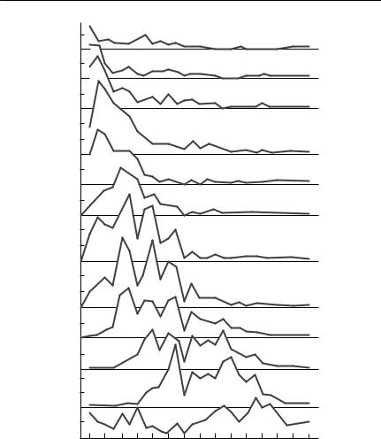
gical and limnological literatures. A full discussion of the possible approaches and problems is beyond the scope of this book. Here I will outline the nature of the problem, discuss why some intuitively appealing methods are flawed, and describe in very broad terms the possible ways forward. Anyone attempting to
128 C H A P T E R 4
use these methods in practice should consult Manly (1989) for entomological examples, and Hairston and Twombly (1985) or Caswell and Twombly (1989) for limnological examples. More recently, Wood (1993; 1994) has developed mathematically sophisticated approaches that should be considered. To date, however, they have not often been applied in practice.
The basic problem in attempting to analyse data of this sort is well summarized by Wood (1994): ‘There were two bears yesterday and there are three bears today. Does this mean that one bear has been born, or that 101 have been born and 100 have died?’ There is insufficient information in a simple record of numbers of individuals in various stages through time to define birth and death rates uniquely. If our bears are marked, we have no problem, but if they are not, it is necessary to make assumptions of some sort about the processes that are operating.
In the limnological literature (for example, Rigler & Cooley, 1974), it has been conventional to estimate the number of individuals entering an instar by dividing the area under a histogram of abundance through time by the stage duration, i.e.
Ni = |
Ai |
, |
(4.12) |
|
|||
|
i |
|
|
where Ni is the number of individuals entering the ith stage, Ti is the stage duration and Ai is the area under the histogram. This would be perfectly sound if the stage duration were known, all individuals entered the stage simultaneously and they suffered no mortality. Equation (4.12) then would express the elementary fact that the height of a rectangle is its area divided by its width. Less trivially, eqn (4.12) is also valid if entry to the stage is staggered, provided again there is no mortality and the stage duration is known, because the total area of the histogram is simply the sum of a series of components nitTi, where nit is the number of individuals entering stage i at time t. Thus,
Ai = ∑nit i = |
i ∑nit = i Ni . |
(4.13) |
t |
t |
|
However, Hairston and Twombly (1985) show that eqn (4.12) may grossly underestimate Ni if there is mortality during life-history stage i. If αi, the rate of mortality in the stage i, is known, they show that it can be corrected for, to yield
Ni |
= |
|
Aiαi |
. |
(4.14) |
|
− exp(−αi |
||||
|
[1 |
i )] |
|
||
The utility of eqn (4.14) is limited, beyond showing that eqn (4.12) produces an underestimate, because stage duration and stage-specific survival are unknown, and are usually the principal parameters of interest, as well as being harder to estimate than Ni itself.

V I T A L S T A T I S T I C S : B I R T H , D E A T H A N D G R O W T H R A T E S 129
An intuitively obvious way of estimating stage duration is the time between the ‘centres of gravity’ of successive cohorts (Rigler & Cooley, 1974), with the ‘centre of gravity’ or temporal mean Mi of cohort i being defined as
∑tn (t)
M = ∑ , (4.15) n
where t is time and ni(t) is the number of individuals in cohort i present at time t. Unfortunately, this simple approach is also invalid if either development times or mortality rates differ between instars (Hairston & Twombly, 1985).
Manly (1990) describes a series of methods that overcome the above difficulties. However, the overparameterization problem remains: to make the methods work, it is necessary to place restrictions on the possible parameter values (for example, it may be necessary to assume that the mortality rate is equal in each stage). Other, more elaborate methods may experience numerical problems in the face of sampling variation, which is a ubiquitous property of all biological data (Caswell & Twombly, 1989).
A method promising to overcome many of these difficulties has recently been developed by Wood (1993; 1994). In principle, the approach is relatively straightforward, but it does involve some quite complicated computation. Here, I will outline the principle, and indicate what sorts of data might be approachable in this way. For computational details, Wood’s original papers should be consulted.
The method is based on the McKendrick–von Forster equation, first presented in Chapter 1,
∂n(a,t) |
+ |
∂n(a,t) |
+ n(a,t)μ(a,t) = 0. |
(4.16) |
|
|
|||
∂t |
∂a |
|
||
Here n(a,t) is the number of individuals of age a at time t, and μ(a,t) is the age-specific death rate at time t. A straightforward rearrangement of eqn (4.16) results in an equation for the age-specific death rate,
|
1 |
|
|
∂n(a,t) |
|
∂n(a,t) |
|
||
μ(a,t) = |
|
|
− |
|
|
− |
|
. |
(4.17) |
|
∂t |
∂a |
|||||||
n(a,t) |
|
|
|
|
|||||
Thus, if the shape of the population surface n(a,t) can be estimated, eqn (4.17) will allow the estimation of the age-specific death rate, and the birth rate as a function of time will simply be n(a,t) evaluated at a = 0.
Unfortunately, estimating the shape of the population surface is a far from trivial exercise. The data available are likely to be estimates of the number of individuals in each of several age classes, at a number of sampling times. This obviously bears some relationship to the value of the population surface at that time, but will always be noisy (that is, subject to sampling error), and will

130 C H A P T E R 4
group age ranges together into stages. More precisely, pij, the number of individuals in stage j on the ith sampling occasion, will be
a j (ti )
pij = n(x,ti )d x + εij. (4.18)
a j−1(ti )
Here, aj(t) is the age at which individuals mature out of stage j at ti, the time of the ith sample, and εij represents the noise.
Wood (1994) proposes a complex numerical procedure that uses eqn (4.18) to extract an estimated population surface R(a,t) from a set of observed pijs. There are two important limitations in this procedure. First, the mortality rate μ(a,t) must change smoothly across stage boundaries. This means that if different life-history stages have very different ecology (as is the case with many insects), the method may fail. Second, the procedure requires that the ages at which stage transitions occur should be known, and that all individuals of a given age make the transition to the next stage after the same maturation time. The method therefore cannot deal with distributed maturation times, although it can handle stage durations that vary through time.
Whether this approach is useful for a wide variety of problems remains to be seen. At this stage, it seems that the computational complexity has prevented its general application.
Methods of last resort
This section describes a series of methods for estimating survival rates that are not ideal. For the estimates to be valid, they require fairly restrictive assumptions about either the population itself or the way in which data are collected from it. Nevertheless, it is often necessary to use models for practical purposes, in the absence of ideal data. Provided the restrictions are kept in mind, these methods may at least provide an estimate of some sort for natural mortality. Unless attributed specifically elsewhere, these methods are taken from Caughley (1977a, pp. 90–5).
Two of the methods rely on the population having a stable age distribution. This concept is explained in more detail in the following chapter. For the purposes of this chapter, it is sufficient to note that if age-specific mortality and fecundity rates remain constant, then, whatever the initial age composition, a population will eventually either grow or decline exponentially at a rate fixed by those mortality and fecundity rates. When it does so, the proportions of individuals in each age class are a function of the mortality and fecundity schedules alone, and do not depend on the initial age distribution. This age distribution that is determined by the mortality and fecundity schedules is called the stable age distribution. In the special case that the population size is

V I T A L S T A T I S T I C S : B I R T H , D E A T H A N D G R O W T H R A T E S 131
constant (r = 0), the stable age distribution is called the stationary age distribution (see Chapter 5 for a more detailed discussion).
It should be clear that reliance on a stable or stationary age distribution is a very restrictive assumption. Not only do the mortality and fecundity schedules need to be constant through time, but they must also have been so for a considerable period of time. The time taken to converge to a stable age distribution is dependent both on the nature of the distributions of the life-history parameters and the initial age distribution, but a reasonable rule of thumb is that it will require at least two or three generations.
Comparison of age structure at successive times
If it is possible to obtain an accurate representation of the age structure of a population at successive time intervals, together with an overall estimate of population size, then survival over the time interval can be estimated, assuming the population is closed. It is obvious that, if the number of individuals in age class x + 1 at time t + 1 is 90% of the size of age class x at time t, then survival of this age class over the interval x to x + 1 must have been 90%. The difficulty with this intuitive approach is that it critically dependent on the age structure of the collected sample being properly representative of the population as a whole. Many, if not most, ways of sampling animal populations are likely to be ageor size-selective. In addition, it is necessary to assume that the population is closed, and that the individuals in the population can accurately be aged.
‘Pick-up’ sample
This method can be used if ages at death have been recorded from a population, usually by ‘picking up’ skulls or skeletal remains (Caughley, 1977a, p. 90). If the remains are an unbiased sample of all individuals that have died (and this is a big ‘if’) and provided the population has a stable age distribution and the rate of increase is known and constant, age-specific survival can be determined. The method has usually been applied in cases where r is assumed to be 0. In this case, the number of carcasses Dx of each age x will be proportional to the age-specific death rate, so that
dx = |
Dx |
|
. |
(4.19) |
∑D |
|
|||
|
|
x |
|
|
If r is not constant, but is known, these death rates need to be corrected via
d ′ = d |
x |
exp(rx). |
(4.20) |
x |
|
|

132 C H A P T E R 4
Standing age distribution
If r is known, and the population has a stable age distribution, then a single unbiased sample from the population at the time of breeding will enable calculation of the age-specific survival curve.
Following the definitions for life-table parameters in Table 4.5 (Caughley’s 1977a notation is slightly different), the number of individuals in the population of age x is Kx. Thus, the proportions of individuals in each age class relative to age class 0 are
kx |
= |
K x |
. |
(4.21) |
|
||||
|
|
K0 |
|
|
This means that an estimate of kx, Nx, can be obtained from estimates of the numbers of individuals in each age class, divided by an estimate of the total number of offspring produced in the birth pulse, K0. Then, provided the Nx can be considered estimates from the stable age distribution,
Ox = Nxerx. |
(4.22) |
Two points should be made about this estimate. First, lx and kx are identical if the rate of increase is 0. Second, it is important that the method be applied only to birth-pulse populations sampled at the time of breeding. If this is not the case, then the number of juveniles (0 + individuals) is not K0: it is K0 times survival from birth to the sampling time. This survival would need to be measured separately.
In practice, there are often problems in estimating survival rates from a sampled age distribution, because the number of individuals in successive age classes may not decrease monotonically. This would lead to some estimated mortality rates being negative. If this problem occurred when an entire population was sampled, it would indicate that the underlying assumption of a stable age distribution was violated. However, in a finite sample, it may merely be an artefact of sampling. Caughley (1977a) suggests smoothing the age distribution so that it is always monotonically decreasing. This approach has been used several times since (e.g. Skogland, 1985; Choquenot, 1993). The smoothing should be applied to counts Kx corrected for the rate of increase in the same fashion as eqn (4.22),
M |
x |
= K |
erx. |
(4.23) |
|
x |
|
|
Caughley suggests two methods for smoothing these corrected frequencies: a polynomial regression of log(Mx) versus x, and fitting a curve of the form
|
M |
x |
|
= a + bx , |
|
Probit |
|
|
(4.24) |
||
|
|
||||
M1 |
|
|
|
||
where a, b and i are constants to be estimated, and Probit(p) is the value of a

V I T A L S T A T I S T I C S : B I R T H , D E A T H A N D G R O W T H R A T E S 133
standard normal deviate that corresponds to the probability p in a cumulative normal distribution. Caughley recommends using eqn (4.24) on post first year survival only. Hence, M1 and not M0 appears in the denomination. Equation (4.24) is more flexible than a polynomial regression, but rather messier to fit. Some statistics packages provide routines for performing probit regression, using maximum likelihood. A logit transformation (ln[ p/(1 − p)]) in place of the probit would probably produce very similar results, and any standard logistic regression routine could be used.
Growth rates
Any model of a size-structured population requires modelling of the growth rate of individuals through time. This problem has been tackled in great detail by fisheries biologists, largely because ‘growth overfishing’ (fishing too hard so that fish are caught too soon when they are still too small) is one of the major practical considerations in fisheries management (Hilborn & Walters, 1992).
The first problem in parameterizing a growth model is to decide on a suitable functional form. There is a plethora of possible functional forms in the fisheries literature (Ricker, 1979; Kaufmann, 1981; Schnute, 1981). Some of these are summarized in Table 4.8. The most commonly used growth model, by a considerable margin, is the von Bertalanffy model (von Bertalanffy, 1938),
l |
= l [1 − e−K(t−t0)]. |
(4.25) |
t |
∞ |
|
Here, lt is the length of an individual at time t, l∞ is the asymptotic length, K is the age-specific growth rate, and t0 is a shift parameter to allow the extrapolated size at age 0 to be nonzero. An additional allometric parameter b is also frequently added, particularly if weight w, rather than length, is modelled:
w |
t |
= w [1 − e−K(t−t0)]b. |
(4.26) |
|
∞ |
|
The general shape of von Bertalanffy growth curves is shown in Figure 4.5. Note that the form in eqn (4.25) cannot generate a sigmoidal curve, whereas eqn (4.26) can do so.
Two quite different sorts of data may be used to estimate a growth function for a population (Francis, 1988). Age–size data consist of records of animal size, together with their age. Recapture data are obtained by measuring, marking, releasing and then recapturing animals, so that the growth over the period at liberty can be measured.
Age–size data can obviously only be used if a means of ageing animals is available. The technical difficulties in ageing wild animals are substantial, but are beyond the scope of this book. Maximum likelihood estimation for any of the models in Table 4.8 is relatively straightforward, provided that the ages are accurate, and that the errors can be assumed to be additive (Kimura, 1980). As I explain in Chapter 2, any nonlinear least squares regression routine will

134 C H A P T E R 4
Table 4.8 Growth functions. In each equation, S represents size; t represents age or time; t0 is a constant of integration; S∞ is the asymptotic size, if it exists, and a, b, c and n are parameters to be estimated. Equations describing indeterminate growth do not reach an asymptotic adult size, whereas those describing determinate growth do
|
Differential |
|
|
||
Function |
equation form |
Name, if any, and comments |
Source |
||
|
|
|
|
|
|
S = exp(b[t + t0]) |
|
dS |
= bS |
Exponential. Indeterminate |
Kaufmann (1981) |
|
|
dt |
growth |
|
|
|
|
|
|
||
|
|
|
|
|
|
S = [ab(t + t0)]1/a |
|
dS |
1−a |
Power. Indeterminate growth |
Kaufmann (1981) |
|
|
|
= bS |
|
|
|
|
|
|
|
|
dt
S = S∞ exp[− exp(−a[t −t0])] |
dS |
= aS(lnS∞ − lnS) |
||||||||||
|
|
|
|
|
dt |
|||||||
|
|
|
|
|
|
|
|
|
|
|
|
|
S = S∞[1 + exp(−a[t + t0])]−1 |
dS |
|
|
|
S |
|
||||||
|
|
|
|
|
|
= aS 1 |
− |
|
|
|
|
|
|
|
|
|
|
|
|
|
|
||||
|
|
|
|
|
dt |
|
|
|
S∞ |
|
||
S = S |
∞ |
[1 − exp(−a[t − t |
0 |
])]b |
dS |
|
S |
1 |
|
|||
|
|
|
b |
|||||||||
|
|
|
|
|
|
= abS |
|
|
∞ |
|
− 1 |
|
|
|
|
|
|
|
|
|
|||||
|
|
|
|
|
dt |
|
S |
|
|
|||
|
|
|
|
|
|
|
||||||
Gompertz. Sigmoid, determinate |
Ricker (1979) |
growth; inflexion point is at t0 |
|
Logistic. Sigmoid, determinate |
Kaufmann (1981) |
growth. Inflexion point is at S∞/2 |
|
Generalized von Bertalanffy. |
Modified from |
Determinate growth. If S is |
Kaufmann (1981). |
length, b is usually set to 1, and |
Called the Pütter |
growth is not sigmoid. If S is |
equation by Ricker |
weight, b ≈ 3, and growth is |
(1979) |
sigmoid |
|
n > 1, c1 > 0, c2 > 0
c2 + K exp(c1(1 − n)t) c1
0 < n < 1, c1 > 0, c2 > 0
c1 − K exp(c1(n − 1)t) c2
dS = c1S − c2Sn dt
dS = c2Sn − c1S dt
Richards. Determinate growth |
Ricker (1979) |
with S∞ = (c2/c1)1/(1−n). The |
|
positive parameter K is a |
|
constant of integration. Inflexion |
|
point is at S = S∞n1/(1−n). More |
|
flexible sigmoid curve than those |
|
above. This form is equivalent to |
|
exponential if c2 = 0 and |
|
equivalent to logistic if n = 2 |
|
Richards. See above. This form |
|
is equivalent to the generalized |
|
von Bertalanffy if n = 1 − 1/b |
|
produce maximum likelihood estimates of the parameters in a nonlinear model, provided the errors are additive, independent and normally distributed with a constant variance. A problem that is likely to occur in growth data is that larger errors may be associated with larger sizes, and thus older animals. A transformation to stabilize the error variance should be applied, if necessary, before using the nonlinear regression procedure. The parameters estimated by this approach are the means of the parameters for all members of the sampled population. In particular, if an asymptotic size is estimated, it is the mean size of ‘old’ individuals in the population, and some animals would be expected to reach a larger size.
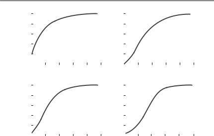
Size
|
|
V I T A L S T A T I S T I C S : B I R T H , D E A T H A N D G R O W T H R A T E S 135 |
||||
100 |
|
100 |
|
|
|
|
|
|
|||||
80 |
|
80 |
|
|
|
|
60 |
|
60 |
|
|
|
|
40 |
|
40 |
|
|
|
|
20 |
|
20 |
|
|
|
|
|
|
|
|
|
|
|
(a)
Size
(c)
0 |
20 |
40 |
60 |
80 |
100 |
0 |
20 |
40 |
60 |
80 |
100 |
||
|
|
|
|
|
|
|
(b) |
|
|
|
|
|
|
100 |
|
|
|
|
|
|
100 |
|
|
|
|
|
|
|
|
|
|
|
|
|
|
|
|
|
|
||
80 |
|
|
|
|
|
|
80 |
|
|
|
|
|
|
60 |
|
|
|
|
|
|
60 |
|
|
|
|
|
|
40 |
|
|
|
|
|
|
40 |
|
|
|
|
|
|
20 |
|
|
|
|
|
|
20 |
|
|
|
|
|
|
|
|
|
|
|
|
|
|
|
|
|
|
|
|
0 |
20 |
40 |
60 |
80 |
100 |
0 |
20 |
40 |
60 |
80 |
100 |
||
|
|
|
Age |
|
|
|
(d) |
|
Age |
|
|
|
|
Fig. 4.5 Examples of growth curves: (a) von Bertalanffy: S∞ = 100, a = 0.05, b = 1, t0 = −5.0;
(b) von Bertalanffy: S∞ = 100, a = 0.05, b = 3, t0 = −5.0; (c) Gompertz: S∞ = 100, a = 0.07, t0 = 15; (d) Logistic: S∞ = 100, a = 0.10, t0 = −30. Units of size and age are arbitrary.
Parameters estimated by recapture methods are not the same as those estimated from age–size data (Francis, 1988). Without an estimate of actual age, it is not possible to place a growth curve on the time axis. What can be done is to estimate the expected growth rate of an individual with an observed size S. It is easy to rearrange the von Bertalanffy equation for length (eqn (4.25) ) into the form
l = (l∞ − l)(1 − exp(−k t)), |
(4.27) |
where t is the time at liberty, |
l is the increase in length, and l is the length at |
first capture. Given a data set including l, l and t for individual animals, it is also easy to fit eqn (4.27) by nonlinear least squares to produce estimates of l∞ and k. The relationship between these estimates and those obtained from fitting eqn (4.25) to age–length data is not straightforward. It has been the topic of continuing debate in the fisheries literature (Sainsbury, 1980; Francis, 1988; James, 1991; Smith et al., 1997). The problem is that fitting eqn (4.27) estimates the expected growth increment of an animal over a period t given that it is of length l at the start of the interval. This is not the same statistical problem as that of estimating the mean growth parameters over all individuals in the population. This point can be illustrated by considering the problem of estimating the asymptotic length l∞. Unless any animals shrink, or unless there is measurement error, l in eqn (4.27) will always be positive, with the result

136 C H A P T E R 4
that the estimated l∞ will be larger than any observed l in the entire data set. This is not the case with estimates of l∞ based on age–length data. (One would expect about half the ‘old’ animals to be larger than l∞.) The solution to this problem depends on the assumptions that are made about the nature of the variability in the growth parameters between individuals in the population. Consult one of the above references for specific advice: the key point is not to expect estimates derived from age–length estimation and recapture data to be directly comparable.
If you want to fit a growth equation other than eqn (4.27) to recapture data, things are more complicated still. The general approach is to solve the differential equation form of the growth equation over a period t, subject to an initial condition that S(0) = S0. For example, consider the form of the Richards equation for 0 < n < 1 in Table 4.8,
dS |
= c |
|
Sn − c S. |
(4.28) |
|
2 |
|||
dt |
1 |
|
||
|
|
|
||
The solution of eqn (4.28) over a period t is also given in Table 4.8, with an integration constant K. If, at time 0, the value of S is S0, then K must solve the equation
S1−n = |
c1 |
− Ke0 |
(4.29) |
|
|||
0 |
c2 |
|
|
|
|
|
K = c1 − S01−n. c2
Hence, when an animal that was initially caught at size S0 was recaptured a period t later, its expected size S t would be the solution of
S1−n = |
c1 |
[1 − (1 − S1−n)exp(c [n − 1] t)]. |
(4.30) |
|
|
||||
t |
c2 |
0 |
1 |
|
|
|
|
|
|
Equation (4.30) is rather messier than eqn (4.27), but, given data on initial and final sizes, together with time intervals, its parameters can be estimated by nonlinear least squares. They will not have the same meaning as parameters fitted to the Richards equation using age–size data.
Stochasticity
Stochastic models, such as population viability analysis models, require an estimate of the probability distribution of survival and fecundity parameters, as well as point estimates. The interval estimates produced by most estimation procedures are based on the sampling distribution of the parameter. In other words, they are a measure of the precision by which the parameter is known, rather than a description of how the value of the parameter varies between

V I T A L S T A T I S T I C S : B I R T H , D E A T H A N D G R O W T H R A T E S 137
individuals through time or across space. In the simple case of a parameter which is normally distributed, there is indeed a straightforward relationship between the estimate of the standard deviation of an estimated mean (its standard error) and the standard deviation of the quantity itself in the general population. This simple relationship does not exist for most of the parameter estimation procedures discussed in this chapter.
A common way to approximate the probability distribution of a parameter is to guess an appropriate value for its coefficient of variation (the standard deviation divided by the mean, and thus a measure of proportional variation), and then to assume that the distribution is of a standard form (usually normal or lognormal). This is, for example, the approach recommended in Burgman et al. (1993). As a first approximation, such an approach is defensible. However, it relies on a usually subjective estimate of the coefficient of variation, and furthermore assumes that a standard probability distribution is adequate. As extinction is often the product of extreme events (Ferson et al., 1989), the tails of distributions are likely to be important, limiting the applicability of standard models.
A second approach is to identify an environmental variable, for which a long time series is available, as the major driver of stochasticity, and then to sample from the time series of that variable to generate stochasticity. This approach has been used for populations in arid areas, in which it can reasonably be assumed that rainfall is the fundamental driver of survival and fecundity (see, for example Bayliss, 1987; Caughley, 1987; McCallum et al., 1995). There are two potential problems here. First, the relationship between rainfall and the parameters of interest may not be well known for endangered species. Second, and more fundamentally, this method assumes that the random variation is white, or uncorrelated variation. Annual rainfall itself may be serially correlated, due to large-scale phenomena such as El Niño (the southern oscillation). More fundamentally, rainfall probably acts on most animal populations via their food supply, introducing both lags and autocorrelation.
Summary and recommendations
1 Fecundity is one of the easier demographic processes to quantify. Data from captive or laboratory populations can be used to estimate clutch or litter size, and age at first breeding. However, the proportion of adult females that breed successfully also determines the mean fecundity of a population. This needs to be estimated from field data. In most modelling contexts, ‘fecundity’ also includes some juvenile mortality.
2 Survival is a difficult process to quantify adequately. Survival of captive animals rarely is a good indicator of survival in the field. Methods to quantify survival can broadly be clustered into life-table methods, which describe
138 C H A P T E R 4
survival through each of a series of life-history stages, and methods using parametric survival curves, which describe survival as a function of age. Consult Table 4.1 for guidance on selecting an appropriate method of analysis.
3 In the absence of reliable data, the inverse of the future life expectancy of an animal of a given age can be used as an estimate of its death rate. Remember, however, that the life expectancy is not the maximum lifespan: it is the mean lifespan.
4 Models of size-structured populations require the modelling of the growth rate of individuals through time. A wide range of growth curves is available in the fisheries literature, as summarized in Table 4.8. Parameter estimates based on age–size data are not directly comparable with those derived from growth increment data.
5 Stochastic models require estimates of the probability distributions of demographic parameters, as well as an estimate of their mean value. A common approach is to estimate the coefficient of variation of the parameter’s distribution, using estimates from several different times or places, and then to use this in a standard probability distribution, such as the lognormal. An alternative approach is to estimate the parameter as a function of an environmental variable, and then to generate the parameter’s distribution by sampling from an existing time series for the environmental variable.