

List of Tables
Table 1.1 |
The GTAP 7 database ............................................... |
7 |
Table 1.2 |
Estimates of the elasticities of substitution between |
|
|
capital and energy (sEK) ............................................ |
17 |
Table 1.3 |
Elasticity of substitution values in each GTAP-E model nest .. . .. |
18 |
Table 1.4 |
Armington elasticities for domestic/imported allocation |
|
|
(ESUBD) and for regional allocation of imports (ESUBM) . . . . . |
19 |
Table 1.5 |
Regional aggregation and countries ................................ |
20 |
Table 1.6 |
Regional blocs and sectoral aggregation ........................... |
21 |
Table 2.1 |
Ad valorem carbon tariffs for alternative scenarios ............... |
38 |
Table 2.2 |
Changes in RCA for the EU and the USA in alternative |
|
|
scenarios .............................................................. |
38 |
Table 2.3 |
Comparing results with a cooperative solution .................... |
39 |
Table 2.4 |
Carbon tax average price impacts in selected countries |
|
|
with a cooperative solution .......................................... |
39 |
Table 2.5 |
Distribution of welfare impacts in a cooperative solution . . . . . . . |
40 |
Table 4.1 |
Recommendations per state and degree of implementation . . . . . . |
67 |
Table 4.2 |
Probit analysis of the decision to implement |
|
|
IAC recommendations ............................................... |
69 |
Table 4.3 |
Probit analysis of the decision—costs and benefits |
|
|
associated with IAC .................................................. |
69 |
Table 4.4 |
State and regional policy tracking definitions ..... .... ..... .... ... |
71 |
Table 4.5 |
US state and regional climate policy ............................... |
74 |
Table 4.6 |
Number of US EPA state and regional climate policies |
|
|
in 2008 ................................................................ |
75 |
Table 4.7 |
Efficacy of the IAC programme in reducing |
|
|
energy consumption .................................................. |
77 |
Table 4.8 |
Energy consumption and GHG emissions .... .... ..... ..... .... ... |
79 |
Table 4.9 |
Analysis of the efficacy of the IAC in reducing |
|
|
GHG emissions ....................................................... |
79 |
Table A.1 |
Summary of data ..................................................... |
81 |
xv
xvi |
List of Tables |
|
Table 5.1 |
Results of the model (T: technology, |
|
|
R: regulation driver, market demand) . . .. . . .. . . .. . .. . . .. . . .. . . .. . |
90 |
Table 5.2 |
Share of stringent regulation triggering innovation . . . . . . . . . . . . . |
92 |
Table 6.1 |
Descriptive statistics ................................................ |
109 |
Table 6.2 |
Baseline results of the effect of policy uncertainty |
|
|
on innovation ........................................................ |
109 |
Table 6.3 |
Tests of robustness ................................................. |
111 |
Table 7.1 |
KLD rating categories .............................................. |
121 |
Table 7.2 |
Allocation of product and process categories ........... ......... |
124 |
Table 7.3 |
Paired sample t-tests: product and process |
|
|
EP—consumer firms ................................................ |
127 |
Table 7.4 |
Paired sample t-tests: product and process |
|
|
EP – industrial firms ................................................ |
129 |
Table 7.5 |
Regression for non-eco CSP, firm type and innovativeness . . . . |
131 |
Table 7.6 |
Overview of results ................................................. |
132 |
Table 7.7 |
Correlation innovativeness and eco-activity . . .. . . . . . . . . . . . . . . . . . |
134 |
Table 7.8 |
Correlation innovativeness and eco-impact . .. .. .. . .. .. .. .. .. .. .. |
135 |
Table 7.9 |
Correlation innovativeness and product-related eco-activity . . . |
136 |
Table 7.10 |
Correlation innovativeness and process-related eco-activity . . . |
137 |
Table 7.11 |
Correlation innovativeness and product-related eco-impact . . . . |
138 |
Table 7.12 |
Correlation innovativeness and process-related eco-impact . . . . |
139 |
Table 8.1 |
Description of variables ............................................ |
151 |
Table 8.2 |
Environmental regulation (CO2 emissions) and energy |
|
|
and resource efficiency innovations (fixed effect estimator) . . . |
152 |
Table 8.3 |
Environmental regulation (acidification) and energy |
|
|
and resource efficiency innovations (fixed effect estimator) . . . |
154 |
Table 9.1 |
Estimates for CO2 emission efficiency . .. .. .. . .. .. . .. .. .. . .. .. . .. |
169 |
Table 9.2 |
Estimates for NOx emission efficiency ........................... |
170 |
Table 9.3 |
Estimates for NMVOC emission efficiency ...................... |
171 |
Table 9.4 |
Estimates for SOx emission efficiency .. .. .. .. .. .. . .. .. .. .. .. .. .. |
172 |
Table 9.5 |
Estimates for CO emission efficiency . .. . .. . .. . .. . .. . .. . .. . .. . . .. |
173 |
Table 10.1 |
Descriptive statistics ................................................ |
196 |
Table 10.2 |
Pooled panel estimations ........................................... |
197 |
Table 10.3 |
Specific technology estimations ................................... |
198 |
Table 11.1 |
Green Inventory classes related to biofuels . .. .. . .. . .. . .. .. . .. . .. |
208 |
Table 11.2 |
Data available on Thomson innovation ........................... |
213 |
Table 11.3 |
Information available in the BioPat database .. .. ... ... .. ... ... .. |
217 |
Table 11.4 |
Selected countries in BioPat for descriptive statistics ........... |
218 |
Table 11.5 |
Count of records and share of patents by main country |
|
|
and patent office .................................................... |
219 |
Table 11.6 |
Validation of BioPat for EPO patents: percentage |
|
|
of patents related to the biofuels sector ........................... |
219 |
Table 11.7 |
Examples of keywords ............................................. |
224 |

Introduction
Valeria Costantini and Massimiliano Mazzanti
Although the environmental economics literature has recently expanded even in less explored realms such as innovation and policy empirical analysis, there is still room and a need for further investigation in a number of directions. Notwithstanding the need to establish and refine economic theory in this realm, it is the applied environmental economics side that offers very interesting advancements. On a general level, there is a need to bring issues and tools closer. Innovation is a keyword in this book and is a good example. Innovation is undoubtedly an established issue in economics and also in environmental-ecological economics studies, and environmental innovation has progressed and affirmed itself as a key factor in recent years. Nevertheless, there is a need for more complex dynamic reasoning. The wider range of dynamic studies will reinforce the environmental economics research agenda and create closer links to fields such as evolutionary economics, areas of business studies, analysis of structural change and regional studies with a focus on innovation. A greater emphasis on dynamic studies on the applied side may also stimulate further, challenging research at theoretical level in environmental and public economics.
We believe that there is value in new studies covering the environmental modelling of economic-environment interactions and policy assessment. In this book, we mainly address four interlinked issues: the potential alternative use of recently available hybrid economic-environmental accounts at meso level, both for ex ante and ex post analysis; the role of dynamics in explaining how economic and environmental systems co-evolve; the specific role of technological innovation as a driver and an outcome of sustainability goals; and the importance of working at sector-based level rather than at aggregated national level.
V. Costantini
Department of Economics, Roma Tre University, Rome, Italy
M. Mazzanti
Department of Economics & Management, University of Ferrara, via Voltapaletto 11, Ferrara, Italy
CERIS CNR Milan, Via Bassini 15, Milan
xvii
xviii |
Introduction |
The generation of new input-output (I-O) tables at European Union (EU) level in recent projects such as EXIOPOL and WIOD is a good development, as well as the excellent releases by Eurostat of a first National Accounting Matrix including Environmental Accounts (NAMEA) for EU in 2011 (Costantini et al. 2012). Efforts in economic-environmental accounting offer rich extensions and potential links to many fields (innovation studies but also mounting studies on international trade effects on the environment according to both consumption and production sustainability). EU environmentally extended I-O and NAMEA will be probably extended in the future, thus generating a powerful arena for dynamic analysis.
The dynamic framework is intrinsically related to ongoing transformations of the economic and environmental systems, with innovation and policy as main levers of changes. Analysis of such a constantly transformed environment is what makes broad and hybrid approaches different from static, very narrow fields. The real challenge today is a deeper analysis and broader understanding of the dynamic world that presents many methodological, theoretical and empirical challenges. After consolidation of static environmental economics theory, dynamic thinking has increasingly emerged since the mid-1990s. The flaws of mainstream economics in dealing with dynamics are known, but heterodox approaches have also failed to recognize full economic-environmental interplays, either by placing emphasis on innovation alone (with no regard for environmental issues) or by focusing on frameworks that are too limited (I-O, decomposition approaches) for these aims. We therefore believe that we need to select a number of different tools from the analytical box in order to enrich and empower the knowledge of dynamic environments: extending the role of innovation in mainstream environmental economics, applying innovation and evolutionary theory even more extensively to ecological-environmental economics, dynamically extending economic-environmental accounts, placing emphasis on the sector and meso level but also interlinking this with micro and macro settings (Dopfer 2012) and developing robust tools for policy evaluation from efficiency and effectiveness perspectives. The amalgamation of tools and thoughts and the intrinsic dynamic development of social phenomena make imagining new perspectives that generate new knowledge and research opportunities necessary. This is the powerful ‘creative power’ of both hybridization attempts and dynamic thinking. We cite Mallarme´, who is quoted at the beginning of a very dynamicminded book in social theory, Reason and Revolution by Marcuse (1966):
Je dis: une fleur! Et, hors de l’oubli ou` ma voix rele`gue aucun contour, en tant que quelque chose d’autre que les calices sus, musicalement se le`ve, ide´e meˆme et suave, l’absente de tous bouquets.
Sector-based analysis is increasingly recognized as the optimal dimension when evolutionary patterns for consumption and production behaviours are under scrutiny.
A few more words on sector analyses and innovation should be added to the above comments on the key issues this book covers in order to offer food for thought for new research.
Introduction |
xix |
Specific sector performances (innovative, environmental and economic) are crucial to the future competitiveness and achievement of environmental targets in the EU. Sector-based interconnections and spillovers at EU level are key drivers as well as the induced innovation effects of environmental policy.
Sector and dynamics are the keywords that amalgamate analyses centred on environmental innovation and policy. It is worth noting that there is special interest on the assessment of if and how ‘shock events’ (e.g. policy, market shocks) influence innovation and environmental dynamics over the medium-long-run trend and whether different sectors present different reactions to these shocks.
The identification and evolution of green sectors on the one hand, and the transformation of brown sectors such as the car industry on the other, is crucial to understanding evolving systems and patterns of change towards sustainability.
Unsustainable production dynamics in fact involve a structural redefinition that sees an increasing role for environmental friendly technologies in both green and brown sides of the economy and industry, in an interconnected perspective, in line with the Porter hypothesis framework (Porter and van der Linde 1995).
It is worth noting that the empirical decompositions of changes in resource use (RU) and pollution highlight that the ‘technology effect’ is the main factor that balances the increase of RU as driven by economic activity, whereas the ‘industry mix’ effect is not the main driver of environmental efficiency gains. The weakness of an industry mix effect may be explained by looking more closely at industrial trends in Europe. Contrary to expectations, from the mid-1990s to the mid-2000s, the EU increased its share in world manufacturing in certain sectors that can be classified as brown economy industries (pulp and paper, petroleum refining, chemicals, basic metals, motor vehicles). This trend is confirmed by specialization indexes and is largely driven by the increased specialization of Germany and the German-centred industrial block comprising Austria and some Eastern European countries.
In addition, the shift towards a service economy does not necessarily lead by itself to sustained GHG reductions. The increasing interdependence between services and industry (each of them activating a significant amount of input provided by the other macro-sector through push and pull multiplier effects) makes even immaterial service sectors heavily dependent on resource-intensive inputs. This applies even more to certain ‘material intensive’ services such as transport: more extensive production networking and the increased role of intermediate goods may lead to higher circulation of goods and higher intensity of transportation. In the end, the indirect emissions accounted for by services may increase more than their total economic effect and account for about 30% of the total, almost on a level with manufacturing.
Given the relevance of sector interdependences, the manufacturing sector cannot be the only focus of analysis when looking at innovation effects in open innovation systems. The increasing role of vertical integration makes it necessary to look at both industry and service industry innovation dynamics.
Moreover, the effects of environmental policy on the innovation system should take into account the increasing share of imported intermediate inputs from
xx |
Introduction |
countries with weaker environmental standards which implies that emissions associated to domestic output are partly leaked abroad through trade. The technology effect in this trade-related perspective is important since it means that both sides of the coin must be examined: how emissions are relocated abroad, but also how trade drives technology shifts/spillovers and green technology can enhance the competitiveness of the EU (Costantini and Mazzanti 2012).
Summing up, this book aims to develop a series of integrated theoretical and empirical approaches which try to deal with the complexity and richness of a dynamic framework. In order to study the role of innovation and environmental policy in determining economic performance, a dynamic framework is unavoidable for both scholars and policymakers. The latter may receive increasing and more robust information on how to shape long-run policy targets and instruments from theory-empirical integrated modelling.
The various works in the book offer a framework for jointly analysing environmental and economic performances from both theoretical and applied perspectives, with a strong policy flavour concerning ex ante and ex post policy effectiveness, mainly conducted at the meso level with a focus on economic competitiveness and patterns of technological change.
The first part of the book is mainly devoted to analysing how to model macroeconomic scenarios in which energy issues, economic performances and environmental policy are jointly investigated. In Chap. 1, a macro-oriented tool is developed using the Global Trade Analysis Project-Energy (GTAP-E) model. A modified version of the standard GTAP-E model is presented in order to provide an accurate analysis tool for the economic and carbon emissions effects related to alternative climate change policies. Regional disaggregation which allows the role of major countries in economic as well as emissions responses to be better identified is performed. The sector disaggregation is closely related to international energy balances in order to calibrate the model on more realistic emission levels. An ad hoc emissions intensity calibration is also implemented for better representation of sector-based emission levels.
The modified GTAP-E model developed in Chap. 1 is then additionally modified in Chap. 2 in order to specifically address international competitiveness issues related to climate change policies. A set of alternative scenarios dealing with carbon border taxes provides evidence of the scarce effectiveness of trade measures in reducing carbon leakage and enhancing economic competitiveness when strong negative welfare effects influence the whole world.
In line with the challenge of integrating dynamics and innovation with environmental issues, in Chap. 3, Del Rio and Bleda analyse the ability of a policy instrument to generate a continuous incentive for technical improvements and cost reductions in technologies in order to assess and choose in long-run scenarios environmental and energy policies where innovation lock-in is relevant.
Narrowing down the focus on the energy sector, while retaining a national perspective, Chap. 4 provides an in-depth analysis of the impact that two US policies have had on energy consumption and carbon emissions of small and medium enterprises (SME). As a main finding, some policies seem to be more
Introduction |
xxi |
effective than others in reducing energy consumption and carbon emissions where there are notable differences across states in climate policy and investment decisions. These considerations bring robust evidence on the convenience of adopting a sector-based approach when complex systems are investigated.
In Chap. 5, Wagner provides an additional analysis tool where firm-level relationships are investigated. Links between sustainability-related regulation and environmental-related innovation are investigated by using case study data and survey data for German manufacturing firms. By studying the interaction of different kinds of regulations with several types of innovation, Wagner finds that innovations triggered by regulation can improve the environmental performance of the affected product and/or related processes and that this leads to innovation offsets which exceed the costs of compliance and enhance competitiveness. This empirical evidence is a strong confirmation of how important the scale of analysis is even if dynamic approaches allowing for recursive effects to be investigated are adopted.
In the second part of the book, we present works that mainly use empirical tools and focus on the possible complementarities between different data sources that are currently available, allowing for policy evaluations as well as shaping dynamic technological patterns.
An example of policy evaluation is offered in Chap. 6 where Kalamova et al. study the role that environmental policy uncertainty can play on innovation in environmental technologies. By using patent data as a proxy for innovation and volatility in public expenditures on environmental RD as a measure of policy uncertainty, support is found for the negative effect of uncertainty on innovation efforts. This is a clear indication of how important policy design is in a dynamic long-run scenario where the alternative forms of regulation may influence innovation, as in Chap. 5, and the overall institutional quality may affect this inducement effect, as in Chap. 6.
Chapter 7 examines the link between environmental performance, corporate social performance and innovativeness for consumer and industrial firms, using company data on R&D, for US-based firms. A positive correlation is found to exist between environment and non-environment social performance in many dimensions and a positive but weak link between environmental performance and R&D per employee or unit of sales.
In Chap. 8, Crespi shows how micro and meso levels can be fruitfully amalgamated by using innovation as a principal component of the glue. The study provides an empirical analysis of the effects of environmental policy on technological innovation in a specific field of environmental technologies. The empirical results show the existence of a robust enhancing effect played by environmental policy on energy and resource efficiency innovations. In addition, the introduction of energy and resource efficiency technologies is found to be positively associated with innovative investment and strictly related to improved product quality.
In Chap. 9, Marin also offers interesting examples of how sector-based applied analyses can enrich the understanding of economic-environment and innovation dynamics. The patterns of emission efficiency growth in manufacturing sectors for
xxii |
Introduction |
European countries are studied where emission efficiency growth is expected to be triggered by an improvement in the efficiency of frontier countries through the diffusion of better technologies to laggard countries.
Patent data for the analysis of invention patterns are exploited in Chaps. 10 and 11. In Chap. 10, Nicolli adopts a patent class approach to developing and exploiting a data set on patents for the waste sector where specific policy drivers are used for shaping the co-evolutions of innovation and policy dimensions.
In Chap. 11, an alternative methodological approach to patent class is proposed to investigate sector-based innovation patterns more thoroughly when innovation output is far from being industry specific. A keyword selection tool is thus implemented by applying a so-called process analysis to the biofuels sector. Interesting information on radical vs. incremental innovation patterns as well as regional differences in innovative specialization provide robustness for the methodological approach proposed here.
We conclude with a policy-oriented reflection. Further exploration of the dynamic evolution of economic and environmental indicators, by focusing on innovation and invention, is one of the main aims and challenges of environmental and ecological economics at present. It is innovation, generated by firms and diffused within and across sectors, that enhances economic and environmental productivities, the only source of sustainable growth/development. In order to fulfil the ambitious targets that our societies have set and will define, we need, above all, a better understanding of how socioeconomic worlds behave in dynamic settings. This knowledge is complementary to policy implementation. Policies supporting innovation are a source of complexity in the study of social phenomena and are finally informed by economic analyses as well. Although knowledge of such complex, interconnected and dynamic social environments is always partial, this is the direction we believe we should take from here on.
References
Costantini, V., & Mazzanti, M. (2012). On the green and innovative side of trade competitiveness?
Research Policy, 41, 132–153.
Costantini, V., Mazzanti, M., & Montini, A. (2012). Hybrid economic environmental accounts. London: Routledge.
Dopfer, K. (2012). The origins of meso economics. Journal of Evolutionary Economics, 22, 133–160.
Marcuse, H. (1966), Ragione e Rivoluzione. Hegel e il sorgere della teoria sociale. Bologna: Il Mulino (first edition 1941, Reason and revolution. Hegel and the rise of social theory. New York: Oxford University Press).
Porter, M. E., & van der Linde, C. (1995). Toward a new conception of the environmentcompetitiveness relationship. Journal of Economic Perspectives, 9, 97–118.
Part I
Modelling Macroeconomic Scenarios:
Energy Issues, Economic Performances
and Environmental Policy

Chapter 1
The GTAP-E: Model Description
and Improvements
Alessandro Antimiani, Valeria Costantini, Chiara Martini, Alessandro Palma, and Maria Cristina Tommasino
Abstract A modified version of the GTAP-E model is developed in order to assess the effects of alternative climate change policies on economic and carbon emissions. We propose regional disaggregation which allows the role of major countries in economic as well as emission responses to be better defined. Sector disaggregation is closely related to international energy balances in order to calibrate the model on more realistic emission levels. An ad hoc emission intensity calibration is also implemented for better representation of sector-based emission levels. A specific analysis on substitution elasticities in the energy nests completes the proposed adjustments to the original GTAP-E model.
Keywords GTAP-E • Climate change policy • Computable general equilibrium model • Substitution elasticity • Energy balances
1.1Introduction
In recent years, the energy-economy system has become an urgent issue to deal with due to growing concerns over climate change, the differentiation of energy sources, energy price volatility, energy supply independence and technological
A. Antimiani
National Research Institute for Agricultural Economics (INEA), Via Nomentana 41, 00161 Rome, Italy
e-mail: antimiani@inea.it
V. Costantini (*) • C. Martini • A. Palma
Department of Economics, Roma Tre University, Via Silvio D’Amico 77, 00145 Rome, Italy e-mail: v.costantini@uniroma3.it; cmartini@uniroma3.it; apalma@uniroma3.it
M.C. Tommasino
Italian National Agency for New Technologies, Energy and Sustainable Economic Development (ENEA), Rome, Italy
e-mail: cristina.tommasino@enea.it
V. Costantini and M. Mazzanti (eds.), The Dynamics of Environmental |
3 |
and Economic Systems: Innovation, Environmental Policy and Competitiveness,
DOI 10.1007/978-94-007-5089-0_1, # Springer Science+Business Media Dordrecht 2013
4 |
A. Antimiani et al. |
progress. Moreover, there is considerable interest in assessing the effectiveness of environmental policy measures. To this aim, applied economics makes large use of complex analytical models that attempt to capture economy-wide impacts, as much as possible.
We can divide these models into two broad categories: bottom-up and top-down models. The first describes energy demand and supply in detail and also allows the most advanced technologies to be incorporated, such as in the Markal-TIMES model (Loulou et al. 2005). On the other hand, top-down models focus on a complete representation of economic world by mapping a large set of sectors and regions. They are particularly suitable for policy evaluations at national and global level in terms of public finance, employment, terms of trade and other macroindicators (Hourcade et al. 2006). Furthermore, after nearly two decades, modelling approaches offering a hybrid methodology began to appear in the mid-1990s (IPCC 1995).
A further important distinction in economic modelling is between computable partial equilibrium and computable general equilibrium models (hereinafter referred to as CPE and CGE models). CPE models assume fixed prices and income in the rest of the economy and include only one or few sectors whereas CGE models allow simultaneous quantification of economic trade-offs, direct effects and indirect spillovers induced by policy changes in a general equilibrium framework and in an inter-temporal and global perspective (Conrad 2001).
1.2Bottom-Up and Top-Down Models
According to Wing (2008), bottom-up models are based on a detailed representation of the productive system as well as the demand side. Based on data on the cost and effectiveness of technologies as well as on basic resources utilisation of a country, such as energy, bottom-up models calculate the optimal mix of technological options on the basis of the cost minimisation principle subject to resource constraints by also taking into account environmental targets such as a CO2 emission cap. This class of models can fully capture specific sectoral features by representing demand and supply complexity, especially in sectors with few market players. In contrast, their weakness is the lack of economic interconnections among markets (sectors) which would evaluate economic effects and feedbacks deriving from a general equilibrium perspective.
Top-down models, on the other hand, describe the economic system as a whole through aggregates and their interrelations in a general equilibrium framework. They put all markets in the economy in Walrasian equilibrium in terms of relative prices, given aggregate factor endowments, households’ consumption behaviour (specified by their utility function) and industries’ output transformation technologies (specified by their production functions). These models usually include
1 The GTAP-E: Model Description and Improvements |
5 |
thousands of equations and variables, both endogenous and exogenous, linked to real world data matrixes.
It is worth noting that top-down and bottom-up models often lead to divergent outcomes when evaluating the impact of policy measures. While top-down models indicate large macroeconomic costs as the consequence of a given mitigation policy, bottom-up models suggest a lower economic response in terms of price distortions, economy-wide interactions and income effects (Wilson and Swisher 1993). The reason for dissimilar results can be found in their different model structure and assumptions. In bottom-up models, the sector-specific focus generates lower costs whereas top-down models capture the costs caused by greater production costs and lower investment in other sectors. Top-down models only capture technology as the share of a given input in the intermediary consumption (usually labour, capital, energy). In CGE models, elasticities are crucial parameters representing the degree of substitutability among inputs and can vary according to different functional forms of the production function.
Recently, a new class of hybrid models has appeared. As their name suggests, these models combine a bottom-up approach – a fully detailed technological frontier representation – with the CGE model equilibrium framework, enriching their capability to represent the real world economy. Hybrid models seem to be more sensitive when assessing policy measures, suggesting higher costs than simple CGE models.
Among the various top-down CGE models, environmental CGE models have assumed special importance by extending the basic economic framework to include the use of natural resources and polluting emissions or other environmental effects associated with the production or consumption of each sector of the economy. As a result, they can be used to estimate the net economic costs or benefits of environmental policies implementing alternative policy measures (e.g. energy taxes or emission trading systems).
A typical CGE model consists of a large set of equations describing model variables and a detailed database that is consistent with the model equations. It usually manages the following types of data:
•Tables of transactions values, usually presented as input-output matrices or social account matrices (SAMs), which cover the economy of countries as a whole and distinguish a number of sectors, commodities, primary factors and types of consumers.
•Elasticity parameters: dimensionless parameters that capture behavioural response among different model actors. Elasticity values, in turn, can be divided in two types: supply and demand parameters. As an example, the supply elasticity parameter called ‘factor substitution’ describes the magnitude with which producers in a sector can substitute inputs (e.g. capital and energy) if their prices ratio changes.
•Tax and tariff rates for each sector and region which allow agents’ prices to be distinguished from market prices.

6 |
A. Antimiani et al. |
1.3The GTAP Model
1.3.1An Overview
A CGE model which has recently shown outstanding growth is the GTAP model. This is part of the Global Trade Analysis Project (GTAP),1 a global network of researchers and policymakers conducting quantitative analysis of international policy issues. The core feature of the GTAP project is a global database including input-output tables on bilateral trade flows, production, consumption and intermediate use of commodities and services as well as transport costs, tax and tariff information. Our decision to use the GTAP model was also driven by its updated and detailed database.
The GTAP model is a multiregional applied general equilibrium model, representing the global economy. In each region, a representative agent maximises utility, and private demand and production are modelled using different functional forms. Some of the most important features that distinguish the GTAP model from other CGE models are the explicit treatment of international trade and transport margins and a global banking sector which intermediates between global savings and consumption. Moreover, the model incorporates a constant-difference-of-elasticity (CDE) utility function in private household preferences. This non-homothetic functional form, unlike the usual homothetic constant elasticity of substitution (CES) function, allows for analysed simulations with large income effect.
1.3.2The GTAP Database
The GTAP 7 database represents the world economy with 2004 as the reference year. All values are expressed in 2004 US dollars, and it covers 57 sectors in 113 regions.2 The 57 sectors included in the GTAP 7 database are defined according to the International Standard Industry Classification (ISIC), except for the agricultural and food processing sectors, which refer to the Central Product Classification (CPC).3
The 113 regions (single countries or groups of countries) are defined as aggregates of 226 countries for which contributors to GTAP database provide domestic data. Table 1.1 synthesises the main sources of the GTAP database version 7.
1Global Trade Analysis Project (GTAP), developed by the Center for Global Trade Analysis in Purdue University’s Department of Agricultural Economics, West Lafaiette, Indiana, USA. For more information, see also https://www.gtap.agecon.purdue.edu/.
2The new GTAP 8 version will be available in 2012 and will allow 2004 and 2007 data to be compared.
3CPC was developed by the Statistical Office of the United Nations to serve as a bridge between the ISIC and other sectoral classification.
1 The GTAP-E: Model Description and Improvements |
7 |
|
Table 1.1 The GTAP 7 database |
|
|
|
|
|
Data source |
Data description and sources |
|
|
|
|
World Bank data |
Macroeconomic aggregates (GDP, private consumption, |
|
|
government consumption and investments) |
|
UN COMTRADE data |
Trade data |
|
OECD PSE/CSE database |
Macroeconomic data (output subsidies, land-based |
|
|
payments, labour and capital-based payments) |
|
WTO and ‘financial report on the |
Macroeconomic data (agricultural exports subsidies) |
|
European Agricultural Guidance |
|
|
and Guarantee Fund’ |
|
|
Market Access Maps (MAcMaps) |
Macroeconomic data (import tariffs) |
|
developed by ITC (UNCTAD- |
|
|
WTO, Geneva) and CEPII (Paris) |
|
|
IMF |
Macroeconomic data (income and factors taxes) |
|
Calibrated from other data sources |
Behavioural information (behavioural parameters such as |
|
|
demand and trade elasticities) |
|
IEA database |
Model Input Energy (primary energy consumption for all |
|
|
113 regions and 57 sectors included in GTAP 7 |
|
|
database) |
|
|
|
|
Source: Narayanan et al. (2008) |
|
|
In the GTAP database, I-O data may be processed in several ways and, if necessary, disaggregated as described in the GTAP database documentation.
Energy is represented by a special set of data, prepared not only to supplement data from sector generic sources but also to ‘correct’ I-O tables. Such an approach has been developed to fix divergences of energy data in earlier GTAP releases from International Energy Agency (IEA) data (see among others, Babiker and Rutherford 1997). With regard to energy flows, the GTAP database includes not only money value but also volume data, referring to I-O tables and international trade flows measured in millions of tons of oil equivalent (Mtoe). In particular, the energy data file contains three arrays that report the volume of energy commodities (viz. coal, natural gas, oil, oil products and electricity) purchased by firms and households and also the volume of bilateral trade in energy commodities.
The main source of energy data is the International Energy Agency ‘Extended Energy Balances’ (IEA EEBs onwards) for 2004. The energy balance constitutes a large array of energy flows, built using a different sectoral classification; in order to be used in the GTAP model, the energy data should be aggregated and harmonised with the rest of the database. Although the EEB classification of energy flows and products is much more detailed than the GTAP, the classification of nonenergy sectors is less detailed in EEBs. Furthermore, unlike the GTAP, IEA EEBs do not recognise gas distribution as a separate activity. For the most part, IEA EEB sectoral classifications are treated as disaggregation of the GTAP sectoral classifications. The exceptions fall into three classes. First, some of the IEA EEB sectors are discarded; these include sectors such as ‘statistical differences’ that represent nothing in the real world but are items of accounting convenience. Second, some of the EEB flows are coherent with GTAP classification but not in

8 |
A. Antimiani et al. |
the intermediate usage block: this is true for production, exports and imports. Third, some EEB flows combine uses that must be separated in GTAP such as gas and crude oil industries, the transport industry and private consumption.
1.3.3Model Structure
The GTAP model includes two different kinds of relationships: accounting and behavioural equations. While the first ensures the balance of receipts and expenditures for every agent in the economy, behavioural equations specify the behaviour of optimising agents (production and demand functions). Given the large number of equations in the GTAP model, providing a synthesis of the theory behind the model is not an easy task. The basic accounting relationships can be better understood with a flow chart.4 The graphical illustration provided in Fig. 1.1 explains the basic structure of the GTAP by focusing on the accounting relationships in a multiregional open economy.
First of all, the regional household collects all income that is generated in the closed economy by each region or composite region which derives from ownership and sales of primary factors of production – capital, skilled and unskilled labour, land and natural resources. According to a Cobb-Douglas utility function, regional income is allocated across three forms of final demand (Fig. 1.1): private household expenditures (PRIVEXP), government expenditures (GOVEXP) and savings (SAVE). The flow associated with savings constitutes the input for production sector. This formulation in terms of regional household preferences is well suited to computing regional equivalent variation as an indicator of the welfare changes caused by different policy scenarios.
The GTAP production structure distinguishes between primary and intermediate factors. Among the primary factors – namely land, skilled labour, unskilled labour, capital and natural resources primary factors, the GTAP model additionally distinguishes between endowment commodities which are perfectly mobile and those that are sluggish to adjust (land and natural resources).
The production function of each sector is modelled through a ‘technology tree’ that contains different levels. At the top level, we find a final production nest in which primary factors and intermediate factors are combined and, at the bottom level, a value-added nest and an intermediate nest where the producer chooses the optimal mix of primary factors and intermediate inputs, respectively. It is worth mentioning that imported intermediate inputs are assumed to be separable from domestically produced intermediate inputs, following the Armington assumption (Armington 1969). Under this approach, imported intermediates are separable from domestically produced intermediate inputs: firms first decide on the sourcing of
4 Hertel and Tsigas (1997) offers a detailed explanation of the theory behind the model, especially with regard to the derivation of the behavioural equations.
1 The GTAP-E: Model Description and Improvements |
9 |
SAVE |
net saving, by region |
PRIVEXP |
private consumption expenditure in region r |
TAXES |
different kind of taxes or subsidies |
GOVEXP |
government consumption expenditure in region r |
VOA |
value of commodity i output in region r at agents' prices |
NETINV |
regional net investment |
VDPA |
domestic purchases, by households, at agents’ prices |
VDGA |
domestic purchases, by government, at agents’ prices |
MTAX |
tax on imports on good i from source r in destination s |
XTAX |
tax on exports on good i from source r in destination s |
VIPA |
import purchases, by households, at agents' prices |
VIGA |
import purchases, by government, at agents' prices |
VDFA |
domestic purchases, by firms,at agents' prices |
VIFA |
import purchases, by firms, at agents' prices |
VXMD |
non-margin exports, at market prices |
Fig. 1.1 Multiregional open economy in the GTAP model and flows denominations (Source: Brockmeier 1996)
their inputs and then, according to the resulting composite import price, determine the optimal mix of imported and domestic goods. The way in which the firm combines production factors to produce its output depends on the assumptions made on separability in the production function. Production technology is assumed to be weakly separable between primary factors of production and intermediate inputs meaning that the elasticity of substitution among any individual primary factor and intermediate input is equivalent. It is assuming this kind of separability that enables production function to be represented as a multilevel production
10 |
A. Antimiani et al. |
function (technology tree): indeed, the above-mentioned common elasticity of substitution enters the fork in the inverted tree at which the primary and intermediate factors are joined.
At the top level of the technology tree, a Leontief production function operates, namely, the elasticity between value added and intermediate factors is zero, and they are combined in fixed proportions that are different for each sector. Hertel and Tsigas (1997) highlighted that the Leontief production function and the hypothesis of constant return of scale make the mix of intermediate factors independent of their prices. The technology tree is further simplified by employing the constant elasticity of substitution (CES) functional form in the value-added and intermediate nests (bottom level). Value added is then produced through a CES function of primary factors of production. Each intermediate input is in turn produced using domestic and imported components (following the Armington assumption) with the technical process described by a CES function. Finally, imported components are a mix of imports from the other regions in the global model, with the technical process again described by a CES. Under the CES functional form, the substitution possibilities within each nest are restricted to a parameter that changes from one sector to another. It should be mentioned that this CES assumption is fairly general in sectors that employ only two inputs but, when assuming that all pairwise elasticities of substitution are equal, represents quite a simplification.
Private consumer optimising behaviour is represented in the GTAP by the CDE (constant difference of elasticity) expenditure function, first proposed by Hanoch (1975). This formulation can be considered more flexible than the commonly used CES/linear expenditure system demand functions. Indeed, the CDE function has the desirable property that the resulting preferences are non-homothetic; they also allow for possible differences in income effects since marginal budget shares of individual goods can vary with income levels. CDE functions are more facilitated in their parameter requirements than functional flexible forms. Moreover, parameters of CDE demand functions can be easily calibrated using historical data on income and own price elasticities even though, with the exception of some special cases of the CDE (e.g. Cobb-Douglas functions), elasticities are not constant. On the contrary, they vary according to expenditure shares and relative prices. For this reason, elasticities are updated with iterations given by the non-linear solution procedure; such an approach also allows a mix of composite consumption of tradable commodities included in the model to be obtained, based on domestic and composite imported goods.
The static version of the GTAP model computes a linearised representation of the accounting relations described; in this form, the equations are implemented in GEMPACK language (Harrison and Pearson 2002) which solves non-linear equilibrium problems via iterations and re-linearisation. The model also provides a wide range of closure options, namely, choosing which variables are exogenous; different closures are associated with different policy experiments, exogenously imposed as shocks. Moreover, partial equilibrium closures are possible, facilitating comparisons with studies developed on partial equilibrium models.
1 The GTAP-E: Model Description and Improvements |
11 |
1.4The GTAP-E Model
Recently, growing research demands for integrated assessment of climate change issues have motivated the construction of different versions of the GTAP model and databases related, for instance, to GHG emissions, land use and biofuels.
The GTAP-E (Burniaux and Truong 2002) is an energy-environmental version of the standard GTAP model which allows for inter-fuel and inter-factor substitution in the production structure of firms and in the consumption behaviour of private households and the government sector. In addition to standard macroeconomic results, GTAP-E captures the effects arising from changes in energy-environmental policy strategies, both in terms of economic and environmental indicators.
The GTAP-E model includes modified treatment of energy demand energy-capital and inter-fuel substitution, carbon dioxide accounting, taxation and emission trading, since it has been specifically designed to be used in the context of greenhouse gases (GHG) mitigation policies. The potential of the GTAP-E in existing debate on climate change is illustrated by some illustrative simulations of the implementation of the Kyoto Protocol (among others, Burniaux and Truong 2002). It represents a topdown approach of energy policy simulation since it estimates the demand of energy inputs in terms of sectoral demand producing detailed macroeconomic projections.
The main change in the GTAP-E compared with the traditional GTAP model is the inclusion of the possibility of energy input substitution in production and consumption, allowing for a more detailed description of substitution possibilities in different energy sources. Energy substitution is incorporated in the GTAP-E model, both in the production and consumption structure. The important issue of capital-energy substitutability vs. complementarily is also explicitly considered.
1.4.1Production Structure
In the standard GTAP model, energy inputs are treated as intermediate inputs (outside the value-added nest) whereas the GTAP-E model incorporates energy directly in the value-added nest. In this case, energy inputs are combined with capital to produce an energy-capital composite; the latter is combined with other primary inputs in a value-added-energy nest using a CES function (Fig. 1.2).
GTAP-E model incorporates energy in the value-added nest in two different steps. First, energy commodities are separated into ‘electricity’ and ‘nonelectricity’ groups, where a substitution elasticity (sENER) operates. The following nest separates nonelectric into coal and non-coal with a specific substitution elasticity (sNELY ) and non-coal into gas, oil and oil-refined products, with a specific substitution elasticity
(sNCOL).
Secondly, energy composite is combined with capital to produce energy-capital composite to be incorporated in the value-added nest. This production structure can be further enriched to include biofuel production (Taheripour et al. 2007) or clean energy technologies as in the ICES model (Bosello et al. 2011).
12 |
A. Antimiani et al. |
|
Output |
|
s = 0 |
Value-added Energy |
Intermediates goods |
sVAE |
(No Energy inputs but with |
energy feedstock) |
Natural Land Labour |
Capital- |
Domestic |
Foreign |
|
|
|
|
||
Resources |
Energy |
|
|
|
|
|
|
||
|
|
|
|
Region |
Unskilled Skilled |
sKE |
|
|
|
|
|
|
|
|
Capita |
Energy |
|
|
|
Non- |
|
sENER |
Electricity |
|
|
|
|||
sNELY |
|
|
|
|
Coal |
Non-coal |
|
|
|
|
|
sNCOL |
|
|
Gas |
Oil |
Petroleum |
|
|
|
|
Products |
|
|
Domestic Foreign |
Domestic Foreign |
Domestic |
Foreign |
|
Region |
|
Region |
Region |
|
Fig. 1.2 The GTAP-E production structure
According to this approach, energy inputs are part of the endowment commodities owned by producers. Capital and energy use mainly depends on the model parameters (elasticity values) and the policy simulated.
1.4.2Consumption Structure
As far as consumption is concerned, the GTAP-E model modifies both private and government consumption. In the standard GTAP model, private and government consumption are separated from private savings.
1 The GTAP-E: Model Description and Improvements |
13 |
Government consumption has a Cobb-Douglas structure (with a substitution elasticity equal to one), where energy commodities are separated from nonenergy commodities by a nested-CES structure.
Household private consumption follows the standard GTAP model, using the constant-difference-of-elasticity (CDE) functional form previously described, but in the second-level nest, the GTAP-E model further specifies the energy composite using a CES functional form. A further significant change in the consumption structure is the possibility of adding carbon tax to private expenditure, as well as to public (government) expenditure, for goods that emit carbon dioxide when used.
1.4.3CO2 Emissions and Related Parameters
The GTAP-E model modifies the standard GTAP database to incorporate CO2 emissions from fossil fuel combustion which are incorporated by region, commodity and use in million tons of carbon. Energy commodities include coal extraction (coa), crude oil (oil) extraction, natural gas extraction (gas), petroleum products (pc), electricity (ely) and gas manufacture and distribution (gdt). CO2 emissions for electricity are equal to zero, as well as for all other nonenergy commodities.
CO2 emission data are based on estimates from Lee (2008), properly adjusted to fit with the compatible GTAP format, which contain CO2 combustion-based emission values from intermediate use and government and private consumption playing a key role in describing the behaviour of energy consumers in facing higher energy prices. As an example, taxes on CO2 emissions would require energy consumers to use less-polluting energy such as natural gas instead of coal. In addition, by using detailed and reliable emission data at regional level, analyses of potential carbon leakage effects can be performed.
1.4.4The GTAP-E Revised Version
A recent revision of the energy-environmental extension of the GTAP-E by Burniaux and Truong (2002) can be found in McDougall and Golub (2007); this is adapted to a wider range of energy-environmental policy scenarios. In particular, improvements are related to different issues such as emission data, emission trading, carbon taxation, revenue from emission trading, production structure and welfare decomposition and will be summarised below.
First, new arrays are added to the data file, showing carbon dioxide emissions by region, commodity and use. This represents another way of using the information which in the standard GTAP-E is represented as energy volume data. In particular, the database contains emissions from firms’ usage of domestic and imported intermediate goods, emissions from households and government consumption of domestic and imported products.

14 |
A. Antimiani et al. |
Moreover, in order to model an emission trading system, blocs of regions trading permits among themselves are identified; a non-trading region is simply a oneregion bloc. Considering the Kyoto Protocol framework where Annex-I countries may operate in an emission trading scheme, Annex-I regions constitute one single bloc whereas the remaining non-Annex regions are considered as individual blocs. To impose or relax emission constraints, a bloc-level power-of-purchases variable is defined, relating regional quota to actual emissions; when emission constraints are in force, this variable is endogenous (whereas emission quotas are exogenous) so that regional emissions and emission quotas are decoupled. When not in force, emission quotas are endogenous (whereas power-of-purchases variable is exogenous) so that regional quotas follow emissions.
An economic environment without emission constraints can be simulated by making the power of emission purchases endogenous and the real carbon tax rate exogenous.5 In this case, there are two options for market and agents’ prices: ad valorem tax and carbon tax. To distinguish them, a new computational level is added, including only non-carbon tax for each usage (referring to firms, private and government consumption of energy goods, domestic and imported). The model also enables carbon tax and emission trading revenues to be computed by region from all sources.
Many more intermediate levels of nesting are added in the production system, combining capital with energy at the top level. To implement this system, a new set of subproducts is defined which includes value-added-energy composite, capitalenergy composite, energy composite, nonelectric energy commodities and non-coal energy commodities. Such a production system enables technological change to be simulated at every level in the nest structure. Furthermore, the set of inputs and substitution elasticities are specified with a high level of detail. A similar approach is adopted for all the other nests in the production system whether the inputs are tradable, endowments, subproducts or any combination thereof.
Due to the previous changes, welfare decomposition is subject to a double modification. First, net emission trading revenues are taken into account, and these contribute to welfare changes. Second, welfare contributions of all forms of input-saving technological changes are summed up in a single variable, including technological changes associated with the energy nests of production function.
It is worth mentioning that although GTAP-E has been specifically designed to be used in the context of GHG mitigation policies, its uses include biofuels (Banse et al. 2008; Hertel et al. 2008; Taheripour et al. 2010), induced tourism demand changes in climate change setting (Berrittella et al. 2007a) and the costs of climate mitigation policies (Nijkamp et al. 2005; Kemfert et al. 2005). The framework has also been used to examine water scarcity (Berrittella et al. 2007b) as well as the economic impacts of a rise in sea levels (Bosello et al. 2007). Lastly, Gan and Smith (2006) utilised the GTAP-E model to investigate the cost competitiveness of woody biomass for electricity production in the USA under alternative CO2 emission targets.
5 The real carbon tax rate is defined as the nominal tax rate deflated by the income disposition price index.
1 The GTAP-E: Model Description and Improvements |
15 |
1.5Model Improvements
1.5.1CO2 Emission Data Calibration
In the modified GTAP-E version (GTAP-E-M onwards) developed in this work, we introduce some changes compared with the latest version by McDougall and Golub (2007).
First of all, some changes concern the data used for this GTAP-E version since we have updated the GTAP-E dataset using the latest version of the GTAP database version 7.1 (base year 2004) as well as the latest version of the combustion-based CO2 emission data provided by Lee (2008) for all the GTAP sectors and regions. It is worth mentioning that we introduced some adjustments to specific sectors and regions where emissions were not consistent with data provided by the main international energy agencies (EIA-DOE and IEA). Since CO2 emission data are assigned to each region/sector on the basis of energy input volumes and emission intensity factors, we analysed country-/sector-specific data in order to understand which factors were driving these distortions the most. We found that the emission intensity factors were indeed much higher than the average for some sectors and regions leading to a substantial overestimation of the corresponding emissions reported in the official IEA data on CO2 emissions from fossil fuel combustion. In order to reduce this bias, we replaced the emission intensity factors for those sectors and regions whose values were out of the range 1/+1 compared with the official IPCC emission intensity factors (Herold 2003). On the basis of these new emission intensity factors, we computed adjusted CO2 emissions, obtaining new values for the sectors/regions characterised by outlier emission factors. The work of Lee (2008) was carefully examined; it describes the procedure implemented to calculate carbon emissions from fossil fuel combustion by users (or sectors) of all the 113 regions as covered in the GTAP 7 database. Based on the GTAP-E energy volume data, Lee followed the Tier one method proposed in the IPCC Guidelines (IPCC 2006) which is based on the different emission factors at the sector level.
When calibrating CO2 emission levels derived from the procedure developed by Lee (2008) to assign CO2 emissions for each region and sector, we used the contribution by Herold (2003) as a benchmark and mostly found good matching in the data although some outliers were found. The methodology we adopted to recognise outliers is as follows.
Let mEFij denotes the average value of each specific i-th energy commodity and j-th sector emission factor (EF); then,
nEF < mEFij 1; EF > mEFij þ 1o ) EF outlier |
(1.1) |
Once we had identified all the outliers, we substituted the mean values in the outliers, instead of their original values, to obtain more consistent emission data.

16 |
A. Antimiani et al. |
Finally, we calculated new emission values by applying Eq. (1.1), and then we included the modified EFij values thus obtaining the same scheme as Lee (2008).
In order to include CO2 emissions in the GTAP-E model, some preliminary changes had to be made to adapt data to model requirements. Since the most recent CO2 emission database does not distinguish between domestic or imported sources, we computed these shares as proportional to the volumes of domestic production and imports, respectively. Such a choice is consistent with the methodological assumptions described in Ludena (2007) where a procedure to elaborate CO2 emission data that are useful for the GTAP-E is described.6
It should be noted that emissions in our version could not account for all other GHG emissions since they only relate to fossil fuel combustion, thus providing a lower bound estimate of total emissions and abatement targets. Even if the missing emissions amounted to 15% of total GHG, the underestimation would be quite homogeneous across regions and sectors with the exception of the agricultural and chemical sectors and would not therefore influence the distributive effects of our simulations.
CO2 emissions are produced by energy consumption by firms, government and private households. These direct emissions are taxed without discriminating between the sources of the energy products. In these sectors, domestic and imported goods are treated alike, and there are no grounds for fearing either carbon leakage or competitive disadvantage of national firms. Indirect emissions, linked to the use of nonenergy intermediate inputs, whose production involved burning fossil energy sources and CO2 emissions, are not taken into account.
1.5.2Updated Substitution Elasticities in the Capital-Energy Nest
It is important to point out that the GTAP-E model includes some of the most important features of existing top-down models related to energy and environment, such as those in the GREEN model (OECD 1992) and the BMR model (Babiker et al. 1997). Indeed, an important issue to consider is the structure of the substitution possibilities among alternative fuels (inter-fuel substitution) and between energy aggregate as a whole and other primary factors, such as labour and capital (fuel-factor substitution). In the GTAP-E model, substitution elasticity values between energy and capital ( sEK ) are crucial when determining the aggregate output related to energy price changes since technology (energy efficiency, capital turnover) has many economic implications on the production input choices; moreover, it also affects carbon emission volume, carbon permit prices and welfare. Despite its considerable importance, there are not many empirical studies on the
6 Following McDougall and Golub (2007) and Ludena (2007), we converted emission data from Gg of CO2, as expressed in Lee (2008), into million tons of carbon.

1 The GTAP-E: Model Description and Improvements |
17 |
Table 1.2 Estimates of the elasticities of substitution between capital and energy (sEK )
|
USA |
USA |
USA |
Europe |
Australia |
|||||
|
|
|
|
|
|
|
|
|
|
|
|
Berndt-Wood (1975) |
Kulatilaka (1980) |
Pindyck (1979) |
Pindyck (1979) |
Truong (1985) |
|||||
|
|
|
|
|
|
|
||||
sEK 3.5 |
1.09 |
|
1.77 |
0.60 |
|
2.95 |
||||
Source: Burniaux and Truong (2002)
sEK parameter, and, in addition, available estimates often indicate nonhomogeneous results. Table 1.2 summarises some studies which attempted to estimate the partial Hicks-Allen elasticities of substitution in different regions.
Consequently, some substitution elasticities – precisely the substitution elasticity between the capital-energy composite and other endowments and the substitution elasticity between capital and energy in every nest related to the energy composite – were replaced with those proposed by Beckman and Hertel (2010), as described in Table 1.3.7
The Armington elasticities were also changed as suggested by Hertel et al. (2007); this specific choice allows for a better assessment of carbon leakage implications since the literature agrees on the crucial role of substitution elasticities in the quantification and geographical distribution of leakage rates (Table 1.4).
1.5.3Model Setting and Baseline
In order to simulate different scenarios in the context of an international agreement for CO2 emission reduction, we decided to hypothesise the implementation of the abatement targets in line with the Kyoto Protocol. To this aim, an aggregation of 21 sectors and 21 regions was identified (Tables 1.5 and 1.6).
With regard to regional aggregation, we considered a ‘full-Kyoto’ framework, with 11 Annex-I countries/regions featuring country-specific CO2 reduction commitments. Moreover, in our disaggregation, we singled out the major emerging economies, including Brazil, China and India, as major players in post-Kyoto negotiates.
As far as sectoral aggregation is concerned, in addition to the energy sectors such as coal, crude oil, gas,8 refined oil products and electricity, we singled out energy-intensive sectors (e.g. cement, paper, steel and aluminium) that are expected to be the main sources of carbon leakage.
Using 2004 data, a 2012 baseline was created based on the GTAP 7.1 database. To this end, we built a business as a usual scenario for emission data assuming slow
7For a comprehensive discussion on substitution elasticities in the energy sector, see Koetse et al. (2008) and Okagawa and Ban (2008), while Panagarya et al. (2001) and Welsch (2008) discuss the role of import demand elasticities in international trade.
8The gas sector in the present aggregation includes the natural gas extraction and gas manufacture and distribution sector.

Table 1.3 Elasticity of substitution values in each GTAP-E model nest
|
sVAE |
|
sKE |
|
sENER |
|
|
sELNE |
|
|
sNCOL |
|
||
|
|
|
|
|
|
|
|
|
|
|
|
|
|
|
Sectors |
GTAP-E-M |
GTAP-E |
GTAP-E-M |
GTAP-E |
GTAP-E-M |
GTAP-E |
|
GTAP-E-M |
GTAP-E |
|
GTAP-E-M |
GTAP-E |
||
|
|
|
|
|
|
|
|
|
|
|
||||
Agriculture |
0.23 |
0.15 |
0.25 |
0.50 |
0.16 |
1.00 |
0.50 |
0.07 |
0.25 |
1.00 |
||||
Fishing |
0.20 |
0.15 |
0.25 |
0.50 |
0.16 |
1.00 |
0.00 |
0.07 |
0.25 |
1.00 |
||||
Cattle |
0.23 |
0.15 |
0.25 |
0.50 |
0.16 |
1.00 |
0.00 |
0.07 |
0.25 |
1.00 |
||||
Forestry |
0.20 |
0.15 |
0.25 |
0.50 |
0.16 |
1.00 |
0.00 |
0.07 |
0.25 |
1.00 |
||||
Coal |
0.20 |
3.99 |
0.00 |
0.00 |
0.00 |
0.00 |
0.00 |
0.07 |
0.00 |
0.00 |
||||
Oil |
0.20 |
0.39 |
0.00 |
0.00 |
0.00 |
0.00 |
0.00 |
0.07 |
0.00 |
0.00 |
||||
Gas |
0.65 |
0.35 |
0.00 |
0.00 |
0.00 |
0.00 |
0.00 |
0.07 |
0.00 |
0.00 |
||||
Oil_pcts |
1.26 |
1.26 |
0.00 |
0.00 |
0.00 |
0.00 |
0.00 |
0.07 |
0.00 |
0.00 |
||||
Electricity |
1.26 |
1.26 |
0.25 |
0.50 |
0.16 |
1.00 |
0.50 |
0.07 |
0.25 |
1.00 |
||||
Min_pcts |
0.90 |
1.19 |
0.25 |
0.50 |
0.16 |
1.00 |
0.50 |
0.07 |
0.25 |
1.00 |
||||
Che_rub_pla |
1.26 |
1.19 |
0.25 |
0.50 |
0.16 |
1.00 |
0.50 |
0.07 |
0.25 |
1.00 |
||||
Met_pcts |
1.26 |
1.19 |
0.25 |
0.50 |
0.16 |
1.00 |
0.50 |
0.07 |
0.25 |
1.00 |
||||
Electr_equip |
1.26 |
1.36 |
0.25 |
0.50 |
0.16 |
1.00 |
0.50 |
0.07 |
0.25 |
1.00 |
||||
Transp_equip |
1.26 |
1.36 |
0.25 |
0.50 |
0.16 |
1.00 |
0.50 |
0.07 |
0.25 |
1.00 |
||||
Machinery_eq |
1.26 |
1.36 |
0.25 |
0.50 |
0.16 |
1.00 |
0.50 |
0.07 |
0.25 |
1.00 |
||||
Motorvehicl |
1.26 |
1.36 |
0.25 |
0.50 |
0.16 |
1.00 |
0.50 |
0.07 |
0.25 |
1.00 |
||||
Food_ind |
1.12 |
1.36 |
0.25 |
0.50 |
0.16 |
1.00 |
0.50 |
0.07 |
0.25 |
1.00 |
||||
Tobac_bever |
1.12 |
1.36 |
0.25 |
0.50 |
0.16 |
1.00 |
0.50 |
0.07 |
0.25 |
1.00 |
||||
Pap_pcts |
1.26 |
1.36 |
0.25 |
0.50 |
0.16 |
1.00 |
0.50 |
0.07 |
0.25 |
1.00 |
||||
Text_leather |
1.26 |
1.36 |
0.25 |
0.50 |
0.16 |
1.00 |
0.50 |
0.07 |
0.25 |
1.00 |
||||
Oth_manufact |
1.26 |
1.36 |
0.25 |
0.50 |
0.16 |
1.00 |
0.50 |
0.07 |
0.25 |
1.00 |
||||
Transport |
1.68 |
1.36 |
0.25 |
0.50 |
0.16 |
1.00 |
0.50 |
0.07 |
0.25 |
1.00 |
||||
Sea_transp |
1.68 |
1.36 |
0.25 |
0.50 |
0.16 |
1.00 |
0.50 |
0.07 |
0.25 |
1.00 |
||||
Air_transp |
1.68 |
1.36 |
0.25 |
0.50 |
0.16 |
1.00 |
0.50 |
0.07 |
0.25 |
1.00 |
||||
Services |
1.35 |
1.36 |
0.25 |
0.50 |
0.16 |
1.00 |
0.50 |
0.07 |
0.25 |
1.00 |
||||
Notes: sVAE ¼ ESUVAMOD; sKE ¼ ELKE; sENTER ¼ ENTER; sNELY = ELNE; sNCOL = ELNCOAL. See Fig. 1.2 for a graphical illustration of the GTAP-E nests and parameters
18
.al et Antimiani .A
1 The GTAP-E: Model Description and Improvements |
19 |
Table 1.4 Armington elasticities for domestic/imported allocation (ESUBD) and for regional allocation of imports (ESUBM)
|
ESUBD |
|
|
ESUBM |
|
Sectors |
GTAP-E-M |
GTAP-E |
|
GTAP-E-M |
GTAP-E |
|
|
|
|
|
|
Agriculture |
2.37 |
2.41 |
4.93 |
4.65 |
|
Fishing |
1.25 |
2.41 |
2.5 |
4.65 |
|
Cattle |
2.85 |
2.41 |
4.12 |
4.65 |
|
Forestry |
2.5 |
2.41 |
5 |
4.65 |
|
Coal |
3.05 |
2.8 |
6.1 |
5.6 |
|
Oil |
2.5 |
30 |
5 |
30 |
|
Gas |
2.5 |
2.8 |
5 |
5.6 |
|
Oil_pcts |
2.1 |
1.9 |
4.2 |
3.8 |
|
Electricity |
2.8 |
2.8 |
5.6 |
5.6 |
|
Min_pcts |
2.31 |
2.32 |
3.9 |
4.57 |
|
Che_rub_pla |
3.3 |
2.32 |
6.6 |
4.57 |
|
Met_pcts |
3.55 |
2.32 |
7.23 |
4.57 |
|
Electr_equip |
4.4 |
2.26 |
8.8 |
5.83 |
|
Transp_equip |
4.3 |
2.26 |
8.6 |
5.83 |
|
Machinery_eq |
4.05 |
2.26 |
8.1 |
5.83 |
|
Motorvehicl |
2.8 |
2.26 |
5.6 |
5.83 |
|
Food_ind |
2.72 |
2.26 |
5.59 |
5.83 |
|
Tobac_bever |
1.15 |
2.26 |
2.3 |
5.83 |
|
Pap_pcts |
3.1 |
2.26 |
6.33 |
5.83 |
|
Text_leather |
3.77 |
2.26 |
7.57 |
5.83 |
|
Oth_manufact |
3.75 |
2.26 |
7.5 |
5.83 |
|
Transport |
1.9 |
2.26 |
3.8 |
5.83 |
|
Sea_transp |
1.9 |
2.26 |
3.8 |
5.83 |
|
Air_transp |
1.9 |
2.26 |
3.8 |
5.83 |
|
Services |
1.91 |
2.26 |
3.8 |
5.83 |
|
|
|
|
|
|
|
Note: Oil_pcts Oil products, Min_Pcts Mineral products, Che_Rub_Pla Chemical, Rubber & Plastic, Met_Pcts Metal products, Electr_equip Electronic equipments, Transp_equip Transport equipments, Machinery_eq Machinery equipments, Food_ind Food industries, Tobac_Bever Tobacco & Beverages, Pap_Pcts Paper products, Text_Leather Textile & Leather, Oth_Manufact Other manufactures, Sea_Transp See transport, Air_Transp Air transport
adoption of clean technologies and economic projections to 2012 based on IMF and World Bank data on actual growth rates after the financial and economic crisis. Several steps were necessary to obtain a consistent 2012 baseline. We first updated the database to 2008, assuming population and gross domestic product as reported by the World Bank and IMF data9 and calibrating the emissions to the most recent IEA CO2 data. The same procedure was adopted to bring the model to 2012.
9 In order to treat regional GDP as an exogenous variable and to shock it, regional technological progress was taken as an endogenous variable.

20 |
|
A. Antimiani et al. |
Table 1.5 Regional aggregation and countries |
||
|
|
|
|
Blocs |
Countries |
|
|
|
1 |
Australia |
Australia |
2 |
Belarus |
Belarus |
3 |
Brazil |
Brazil |
4 |
Canada |
Canada |
5 |
China |
China |
6 |
Croatia |
Croatia |
7 |
USA |
USA |
8 |
Swiss |
Swiss |
9 |
Turkey |
Turkey |
10 |
FSU |
Former Soviet Union |
11 |
India |
India |
12 |
Japan |
Japan |
13 |
New Zealand |
New Zealand |
14 |
Norway |
Norway |
15 |
ENEEXP |
Indonesia, Malaysia, Mexico, Argentina, Bolivia, Colombia, Ecuador, |
|
|
Venezuela, Kazakhstan, rest of FSU, Azerbaijan, Iran Islamic Republic |
|
|
of, rest of Western Asia, Egypt, rest of North Africa, Nigeria, Central |
|
|
Africa, south central Africa, South Africa |
16 |
EU |
Austria, Belgium, Cyprus, Czech Republic, Denmark, Estonia, Finland, |
|
|
France, Germany, Greece, Hungary, Ireland, Italy, Latvia, Lithuania, |
|
|
Luxembourg, Malta, Netherlands, Poland, Portugal, Slovakia, Slovenia, |
|
|
Spain, Sweden, United Kingdom, Bulgaria, Romania |
17 |
Rest of Africa |
Morocco, Tunisia, Senegal, rest of Western Africa, Ethiopia, Madagascar, |
|
|
Malawi, Mauritius, Mozambique, Tanzania, Uganda, Zambia, |
|
|
Zimbabwe, rest of Eastern Africa, Botswana, rest of South African |
|
|
Customs |
18 |
Rest of America |
Rest of North America, Chile, Paraguay, Peru, Uruguay, rest of South |
|
|
America, Costa Rica, Guatemala, Nicaragua, Panama, rest of Central |
|
|
America, Caribbean |
19 |
Rest of Asia |
Rest of Oceania, Korea, Taiwan, rest of East Asia, Cambodia, Lao People’s |
|
|
Democratic Republic, Philippines, Singapore, Thailand, Viet Nam, rest |
|
|
of Southeast Asia, Bangladesh, Pakistan, Sri Lanka, Kyrgyzstan, |
|
|
Armenia, rest of South Asia |
20 |
Rest of EFTA |
Rest of EFTA |
21 |
Rest of Europe |
Albania, rest of Eastern Europe, rest of Europe, Georgia |
|
|
|
Notes: We defined ENEEXP (ENergy EXPorting countries) those countries whose fuels export share absorbs more than the 10% of the total exports, according to World Bank data
In both cases, while the emission level in aggregate was correct, its distribution in terms of emission quota among regions was not satisfactory. Consequently, in the 2008 baseline, we corrected CO2 emissions to fit the IEA data whereas in the 2012 baseline, we calibrated the CO2 emissions to the IEA projections.10
10 Emissions were swapped with technical progress using a specific closure (Altertax) that allows some data to be changed but preserves the overall consistency of the model.

1 The GTAP-E: Model Description and Improvements |
21 |
||
Table 1.6 Regional blocs |
|
|
|
Regions |
Sectors |
||
and sectoral aggregation |
|||
|
|
||
Bloc Annex I |
Agriculture |
||
|
|||
|
EU |
Chemical, rubber, plastic |
|
|
USA |
Coal |
|
|
Australia |
Crude oil |
|
|
Canada |
Gas |
|
|
Japan |
Oil products |
|
|
New Zealand |
Electricity |
|
|
Norway |
Metal products |
|
|
Swiss |
Paper products |
|
|
Croatia |
Electrical equipment |
|
|
Belarus |
Food industry |
|
|
FSU |
Machinery equipment |
|
|
Bloc non-Annex I |
Motor vehicles |
|
|
Brazil |
Textile and leather |
|
|
China |
Transport equipment |
|
|
India |
Other manufacturing |
|
|
Mexico |
Transport |
|
|
South Africa |
Sea transport |
|
|
Energy exporters |
Air transport |
|
|
Rest of Africa |
Services |
|
|
Rest of America |
|
|
Rest of Asia
Rest of Europe
1.6Conclusions and Future Research Steps
The carbon emissions in the baseline from 2004 to 2008 computed in our version of the GTAP-E model, which includes the changes in emission intensity factors and substitution elasticities, are much more consistent with those provided by IEA. The improvement obtained is quite substantial since the standard GTAP-E model provides aggregate results that in some cases are at odds with current data. As a result, we are confident that our specification is able to provide a more accurate assessment of the potential extent of carbon leakage.11
It is important to point out that CO2 emissions in the GTAP-E model, as well as the IEA data, refer to fossil fuel emissions only, excluding all other possible CO2 equivalent emission sources. As a consequence, we recomputed the 1990 emission levels in order to get consistent CO2 emission targets in the implementation of
11 Robustness checks for model results to different parameters were addressed by a sensitivity analysis in which standard deviation from results in our version is rather small. More importantly, we also found that by relying on original GTAP 7.1 substitution elasticities, carbon leakage would result in overestimated values, especially due to substitution elasticity between capital and energy in the first nest under the production function.

22 |
A. Antimiani et al. |
Kyoto Protocol commitments.12 Even if our ultimate goal is not to provide realistic CO2 projections but to compare the economic effects of alternative policy scenarios, it is worth emphasising that Annex-I emissions in our baseline are almost identical to those proposed by IEA and reported in the most recent European Environment Agency Report.
Future steps for improving this GTAP-E version will be to model non-CO2 GHG emissions as provided by the GTAP data source by transforming them with I-O tables into emissions subject to carbon taxation compatible with actual CO2 emission from fossil fuel combustion. This means that non-CO2 emissions that are now available and mainly related to final output should be transferred to consumers and firms in the form of productive inputs in order to implement a homogenous carbon tax.
Secondly, it could be helpful to shape the functioning of the emission trading system better by disentangling sectors participating or not in the carbon market and implementing an auctioning system for permits allocation rather than the current grandfathering system which seems to be less efficient.
Acknowledgements The authors wish to thank Giancarlo Tosato and Maria Rosa Virdis for their comments and suggestions. This work has been supported by the research network ENEA-INEA-UNIROMA TRE on integrating bottom-up and top-down energy models: the case of GTAP-E and Markal TIMES-Italy.
References
Armington, P. S. (1969). A theory of demand for products distinguished by place of production.
International Monetary Fund Staff Papers, 16, 159–176.
Babiker, M., & Rutherford, T. (1997). Input-output and general equilibrium estimates of embodied carbon: A dataset and static framework for assessment (Economics Discussion Paper 97-02). Boulder: University of Colorado.
Babiker, M. H., Maskus, K. E., & Rutherford, T. F. (1997). Carbon taxes and the global trading system (Working Paper 97-7). Boulder: University of Colorado.
Banse, M., van Meijl, H., Tabeau, A., & Woltjer, G. (2008). Will EU biofuel policies affect global agricultural markets? European Review of Agricultural Economics, 35(2), 117–141.
Beckman, J. F., & Hertel, T. W. (2010). Validating energy-oriented CGE models (GTAP Working Paper N 54). West Lafayette: Purdue University.
Berrittella, M., Certa, A., Enea, M., & Zito, P. (2007a). An analytic hierarchy process for the evaluation of transport policies to reduce climate change impacts (Working Papers, 2007-12). Milan: Fondazione Eni Enrico Mattei (FEEM).
12 In order to make emission levels in GTAP-E model as consistent as possible with those considered for the Kyoto targets by official IPCC documents, we first calculated the deviation between GTAP-E and IPCC emission data in 2004 and then proportionally changed the 1990 IPCC emission data in order to obtain the effective abatement efforts required by the achievement of the Kyoto Protocol targets.
1 The GTAP-E: Model Description and Improvements |
23 |
Berrittella, M., Rehdanz, K., Tol, R. S. J., & Zhang, J. (2007b). The impact of trade liberalisation on water use: A computable general equilibrium analysis (Working Papers FNU-142). Hamburg: Research unit Sustainability and Global Change, Hamburg University.
Bosello, F., Roson, R., & Tol, R. S. J. (2007). Economy-wide estimates of the implications of climate change: Sea-level rise. Environmental and Resource Economics, 37, 549–571.
Bosello, F., Campagnolo, L., Eboli, F., Parrado, R., & Portale, E. (2011). Extending energy portfolio with clean technologies in the ICES model. Paper presented at the 14th annual conference on global economic analysis, Venice, Italy.
Brockmeier, M. (1996). A graphical exposition of the GTAP model (GTAP Technical Paper). West Lafayette: Center for Global Trade Analysis, Purdue University.
Burniaux, J. M., & Truong, T. (2002). GTAP-E: An energy-environmental version of the GTAP model (GTAP Technical Paper N 16). West Lafayette: Purdue University.
Burniaux, J. M., Martin, J. P., Nicoletti, G., & Oliveira-Martins, J. (1992). GREEN – A multisector, multi-region dynamic general equilibrium model for quantifying the costs of curbing CO2 emissions: A technical manual (OECD Economics Department Working Papers, No.116). Paris: OECD.
Conrad, K. (2001). Computable general equilibrium models for environmental and resource economics. The international yearbook of environmental and resource economics 2002/2003. T. Tietenberg & H. Folmer (Eds.), 66–114. Edward Elgar Publishing: Northampton.
Gan, J., & Smith, C. T. (2006). A comparative analysis of woody biomass and coal for electricity generation under various CO2 emission reductions and taxes. Biomass and Bioenergy, 30, 296–303.
Hanoch, G. (1975). Production and demand models with direct or indirect implicit additivity.
Econometrica, 43, 395–419.
Harrison, W. J., & Pearson, K. R. (2002). GEMPACK user documentation. Melbourne: Centre of Policy Studies, Monash University.
Herold, A. (2003). Comparison of CO2 emission factors for fuels used in greenhouse gas inventories and consequences for monitoring and reporting under the EC emissions trading scheme. European Topic centre on Air and Climate Change (ETC/ACC). Technical Paper 10
Hertel, T. W., & Tsigas, M. (1997). Structure of GTAP. In Global trade analysis, modelling and applications. Cambridge: Cambridge University Press.
Hertel, T. W., Hummels, D., Ivanic, M., & Keeney, R. (2007). How confident can we be of CGE-based assessments of free trade agreements? Economic Modelling, 24, 611–635.
Hertel, T. W., Dileep, B., & Tyner W. E. (2008). Impact of biofuel production on world agricultural markets: A computable general equilibrium analysis (GTAP Working Papers 2413). West Lafayette: Center for Global Trade Analysis, Department of Agricultural Economics, Purdue University.
Hourcade, J. C., Jaccard, M., Bataille, C., & Ghersi, F. (2006). Hybrid modelling: New answers to old challenges. Energy Journal, Special Issue II– Hybrid Modeling of Energy Environmental Policies, 1–12.
IPCC. (1995). Climate change, 1995: Economic and social dimensions of climate change.
Contribution of Working Group II to the Second Assessment Report of the Intergovernmental Panel on Climate Change, International Panel on Climate Change (IPCC), Ch. 8, Cambridge, 1996.
IPCC. (2006). 2006 International panel on climate change guidelines for national greenhouse gas inventories, Vol. 2, Energy, Institute for Global Environmental Strategies (IGES). Hayama: Japan on behalf of the IPCC.
Kemfert, C., Kohlhaas, M., Truong, T., & Protsenko, A. (2005). The environmental and economic effects of European emissions trading (Discussion Papers No. 533). Berlin: German Institute for Economic Research (DIW).
Koetse, M. J., de Grooot, H. L. F., & Florax, R. J. G. M. (2008). Capital-energy substitution and shifts in factor demand: A meta-analysis. Energy Economics, 30, 2236–2251.
24 |
A. Antimiani et al. |
Lee, H. (2008). An emissions data base for integrated assessment of climate change policy using GTAP (GTAP Working Paper 1143). West Lafayette: Center for Global Trade Analysis, Purdue University.
Loulou, R., Remne, U., Kanudia, A., Lehtila, A., & Goldstein, G. (2005). Documentation for the TIMES Model PART I. Wien: Energy Technology Systems Analysis Programme.
Ludena, C. (2007). CO2 emissions in GTAP-E: Ready-for-aggregation GTAP 6.0 data. (GTAP Technical Paper). West Lafayette: Center for Global Trade Analysis, Purdue University.
McDougall, R., & Golub, A. (2007). GTAP-E release 6: A revised energy-environmental version of the GTAP model (GTAP Technical Paper No. 15). West Lafayette: Center for Global Trade Analysis, Purdue University.
Narayanan, B., Dimaranan, B. V., & McDougall, R. (2008). Ch. 2: Guide to the GTAP Data Base. In B. G. Narayanan & T. L. Walmsley (Eds.), Global trade, assistance, and production: The GTAP 7 data base. West Lafayette: Center for Global Trade Analysis, Purdue University.
Nijkamp, P., Wang, S., & Kremers, H. (2005). Modeling the impacts of international climate change policies in a CGE context: The use of the GTAP-E model. Economic Modelling, 22, 955–974.
Okagawa, A., & Ban, K. (2008). Estimation of substitution elasticities for CGE models (Discussion Papers in Economics and Business n 8–16). Osaka: Graduate School of Economics and Osaka School of International Public Policy (OSIPP), Osaka University.
Panagarya, A., Shah, S., & Mishra, D. (2001). Demand elasticities in international trade: Are they really low? Journal of Development Economics, 64, 313–342.
Taheripour F., Birur D., Hertel, T. W., & Tyner, W. (2007). Introducing liquid biofuel into the GTAP database (GTAP Research Memorandum No. 11). West Lafayette: Center for Global Trade Analysis, Purdue University.
Taheripour, F., Hertel, T. W., Wallace, E., Tyner, W., Beckman, F., & Birur, D. K. (2010). Biofuels and their by-products: Global economic and environmental implications. Biomass and Bioenergy, 34, 278–289.
Welsch, H. (2008). Armington elasticities for energy policy modeling: Evidence from four European countries. Energy Economics, 30, 2252–2264.
Wilson, D., & Swisher, J. (1993). Exploring the gap: Top-down versus bottom-up analyses of the cost of mitigating global warming. Energy Policy, 21, 249–263.
Wing, S. (2008). The synthesis of bottom-up and top-down approaches to climate policy modelling: Electric power technologies and the cost of limiting US CO2 emissions. Energy Economics, 31, 547–573.

Chapter 2
Carbon Leakage and Trade Adjustment Policies
Alessandro Antimiani, Valeria Costantini, Chiara Martini, Luca Salvatici, and Maria Cristina Tommasino
Abstract A modified version of the CGE GTAP-E model is used to assess economic and carbon emission effects related to alternative policy measures implemented to reduce carbon leakage. We explore a set of scenarios and compare solutions where Kyoto Annex I countries introduce carbon border taxes based on domestic carbon tax in order to solve the carbon leakage problem unilaterally and solutions where carbon border taxes are determined according to specific objectives. Results provide evidence of the scarce effectiveness of trade measures in reducing carbon leakage and enhancing economic competitiveness and the strong negative welfare effects they have not only on non-Annex countries but also on some Annex I countries.
Keywords Climate change policy • Carbon leakage • Computable General Equilibrium Model • Carbon border tax • Competitiveness
A. Antimiani
National Research Institute for Agricultural Economics (INEA), Via Nomentana 41, 00161 Rome, Italy
e-mail: antimiani@inea.it
V. Costantini (*) • C. Martini • L. Salvatici
Department of Economics, Roma Tre University, Via Silvio D’Amico 77 00145 Rome, Italy e-mail: v.costantini@uniroma3.it; cmartini@uniroma3.it; lsalvatici@uniroma3.it
M.C. Tommasino
Italian National Agency for New Technologies, Energy and Sustainable Economic Development (ENEA), Rome, Italy
e-mail: cristina.tommasino@enea.it
V. Costantini and M. Mazzanti (eds.), The Dynamics of Environmental |
25 |
and Economic Systems: Innovation, Environmental Policy and Competitiveness,
DOI 10.1007/978-94-007-5089-0_2, # Springer Science+Business Media Dordrecht 2013
26 |
A. Antimiani et al. |
2.1Introduction
In recent years, a large body of the international literature as well as policy debate have expressed increasing interest in measures taken to mitigate the negative externalities of climate change policies such as the carbon leakage effect (OECD 2006). The imposition of stringent climate policies may produce substantially distortive effects in terms of displacement of production processes from countries with abating policies (e.g. carbon tax or emission trading) to countries where no climate policies are in force.
Consequently, some forms of border adjustments have been invoked in order to restore a level playing field between domestic producers and foreign exporters (Moore 2010; Wooders and Cosbey 2010).
We will elaborate on the existing studies providing further evidence of the extent of carbon leakage and the impact of different forms of carbon border tax (CBT). The major focus of this chapter is on the ambiguities surrounding the possible goals to be achieved through CBT.
In order to assess the potential economic and carbon emission effects related to CBT adjustment schemes, we use a modified version of the computable general equilibrium GTAP-E model (Burniaux and Truong 2002; McDougall and Golub 2007) described in Chap. 1. We model the pursuit of the Kyoto objectives, depicting a world where two groups exist, abating and non-abating countries. Our regional aggregation includes the 11 Annex I countries/regions with CO2 emission reduction commitments in the Kyoto Protocol and the largest emerging economies within the non-Annex list, including Brazil, China, India and Mexico. In terms of sectoral aggregation, we distinguish 21 sectors in order to simulate the impact of alternative policies in energy-intensive and non-intensive sectors.
In order to build a benchmark for investigating the effectiveness of alternative forms of CBT, we first assess carbon leakage implied by an international emission reduction agreement such as the Kyoto Protocol by modelling two scenarios with and without emission trading. We then compare a cooperative scenario featuring global emission trading with several approaches that introduce different carbon tariff schemes to deal with the carbon leakage effect (hereafter referred to as non-cooperative scenarios).
In the cooperative scenario, Annex I countries face the emission targets defined in the Kyoto agreement whereas non-Annex countries are constrained to a zero increase in domestic emissions. By contrast, in the non-cooperative scenarios, exogenous carbon tariffs are based on the domestic carbon tax or are endogenously computed as ad valorem equivalents required to achieve predetermined objectives. In the former case, carbon tariffs are computed by multiplying the carbon tax either by the actual carbon content of imports or by the carbon content of the corresponding domestic good. In the latter case, the ad valorem tariff equivalent is either set with the aim of eliminating (or at least reducing) the carbon leakage or with the aim of maintaining the competitiveness of Annex I countries.
2 Carbon Leakage and Trade Adjustment Policies |
27 |
The economic and environmental effects resulting from alternative trade adjustment policies are compared with the results from the cooperative zero-leakage scenario. A comparison of this type highlights the advantage for non-Annex countries of changing their conservative position in the climate negotiations.
2.2Carbon Leakage as a Side Effect of Climate Policies
2.2.1A Definition of Carbon Leakage
Cancu`n negotiations in 2010 and Durban COP17 in 2011 represented a step forward for reaching a cooperative solution, but global international cooperation for fighting climate change still seems to be a difficult goal to achieve. Policy actions to reduce greenhouse gas (GHG) emissions remain unilateral and could be undermined by the presence of carbon leakage (Hamasaki 2007). Moreover, these policies are likely to have negative impacts on the international competitiveness of some industrial sectors (OECD 2003, 2005; Veenendaal and Manders 2008).
The vast and growing literature on this issue distinguishes two typologies of leakage. The first one is caused by a shift in the location of production towards noncompliant regions, and the second one is related to an increase in energy consumption in non-abating regions due to lower prices on the international markets resulting from the reduced demand for fossil fuels in abating countries.
The pollution haven hypothesis (Copeland and Taylor 2004) explains the first type of leakage. When countries have different environmental regulatory stringency, production will be located where environmental costs are lower.
The second type of leakage can be explained by referring to the energy market model: the reduction in fossil fuel demand in abating countries leads to lower prices on the world energy markets which in turn fosters energy demand in non-abating countries (Burniaux and Oliveira 2000; Felder and Rutherford 1993).
As a matter of fact, the intensity of the taxing countries’ energy demand combined with the elasticity of the energy supply curve are key drivers in determining different types of leakage. According to Gerlagh and Kuik (2007), the energy market model seems to be the prevalent explanation of carbon leakage estimates from simulation analyses.
The rate of carbon leakage is usually computed as the ratio between the increase of CO2 emissions in non-abating countries and the reduction of CO2 emissions in countries implementing GHG abatement policies. As reported by the Energy Modeling Forum (2000) and Kuik and Verbruggen (2002), carbon leakage rates vary widely (between 5 and 35 %, approximately) according to the model used.
Even if the implications for international trade of emission abatement policies are crucial, especially when considering their acceptability and feasibility, few studies have adopted a global approach and tried to quantify simultaneously the effects on emissions, sectoral exports, output and distributional welfare effects at country and global level (Haaparanta et al. 2001; McKibbin et al. 1999).

28 |
A. Antimiani et al. |
Carbon leakage estimates seem to be very sensitive to different model settings. Two key parameters emerge as the driving factors of highly heterogeneous leakage rates: the Armington elasticities in the import demand module and the substitution elasticities in the energy nests of the production module (Gerlagh and Kuik 2007). If Armington elasticities are low, there will be fewer opportunities for non-Annex countries to expand their exports towards compliant countries, and carbon leakage will be low. As a consequence of price impacts of emission reduction targets, nonabating countries will import less carbon-intensive commodities from Annex I countries. At the same time, given a certain value of Armington elasticities, nonabating countries will easily substitute imported intermediates from Annex I countries with intermediates from other non-abating countries or intermediates produced domestically (Wang et al. 2009), creating a demand-driven leakage effect. In this respect, higher substitution elasticities in the production function between energy and other inputs, as well as between alternative fossil fuels, would lead to larger drops in world energy price and hence to larger leakage rates (Kuik 2001).
2.2.2How to Design Carbon Border Tax Adjustments
Abating countries may decide to impose two forms of CBT: full or partial adjustment. Full adjustment refers to a carbon tariff applied to imported goods from noncompliant countries plus a tax rebate for domestic goods that are exported. Partial adjustment refers to the application of a carbon border tax without rebates on exports (Fischer and Fox 2009).1
There is a growing concern over CBT as a feasible and effective unilateral policy measure for preventing carbon leakage. In particular, three major issues arise from the international literature. The first is how to design a CBT which is consistent with WTO rules, feasible in its implementation and effective in achieving its goal(s). While the carbon price in the abating country is the obvious choice as far as the value of the specific tariff is concerned, there are different opinions about how to quantify the embedded carbon in traded goods from non-compliant countries. Two alternative computation methods are often proposed. The first method applies to imported goods coming from non-abating economies where the carbon content for each good produced is given by the best available technology (BAT) in the abating country Dong and Whalley (2009), whereas the second one considers the effective carbon content of the imported goods, thus relying on the production technique applied by the producing country.
Moreover, if a direct accounting approach is considered, only carbon emissions related to the production process are accounted for. If an indirect accounting approach is implemented, all CO2 emissions related to the production process of all intermediates are considered for the application of the CBT, leading to substantially
1 In the rest of this chapter, the terms carbon tariff or carbon border tax will be used interchangeably.
2 Carbon Leakage and Trade Adjustment Policies |
29 |
higher implementation difficulties. Choosing the indirect emission accounting approach strongly affects carbon leakage estimates, as is shown in Atkinson et al. (2010) where the carbon tariff equivalent to a carbon price of 50$ per ton of CO2 amounts to 10 % of the value of the average export bundle of non-abating countries, and tariffs may be two to three times higher for specific sectors.
The second issue concerns the effectiveness of CBT in preventing carbon leakage (Schenker and Bucher 2010). Empirical analyses provide contrasting results on the capacity of CBTs to reduce emissions from non-abating countries, depending both on model settings and alternative CBT designs (Dong and Whalley 2008; Mattoo et al. 2009).
A third issue relates to welfare implications of a CBT approach. The degree of political acceptance of a policy is very likely to depend on its welfare distribution effects for the different economic agents or countries affected by its implementation. CBTs clearly represent a second best solution compared with the implementation of global climate policies which would establish a uniform carbon price for all countries (Stern 2006).
2.3Scenario Setting
The rate of carbon leakage is defined as the increase in CO2 emissions in the rest of the world induced by the domestic reduction measures as a percentage share of the absolute value of the volume of CO2 reduction obtained by compliant countries, according to the following equation:
CLR ¼ |
DCO2Non Annex |
|
DCO2Annex 100: |
(2.1) |
We first check the existence of carbon leakage in a pure Kyoto Protocol scenario, where we impose reduction targets on all Annex I countries with respect to their 1990 emission levels, as if the United States had also ratified the protocol. In particular, we assess the existence of carbon leakage both allowing for the possibility of emission trading among Annex I countries (ET scenario) and only implementing domestic measures (NO-ET scenario).2 An adjustment of emission targets was needed since the high amount of emission permits potentially supplied by transition economies in Annex I (the FSU and Belarus in our model) would result in a close-to-zero carbon price.3
2The emission trading is modelled assuming that all abating policies can be expressed in monetary values by computing a domestic carbon tax that is applied to fossil fuel consumption. The carbon tax equals the equilibrium permits price when emission trading is introduced. This approach, which is common practice in general equilibrium modelling, enables the relative incidence of the compliance costs among countries to be assessed.
3This problematic issue refers to the so-called hot air debate and also addresses the role of the other flexible mechanisms required by the protocol (World Bank 2010). Consequently, for FSU and Belarus, the 0 % target scheduled in the protocol is applied to the emission levels in 2012 rather than the 1990 period.
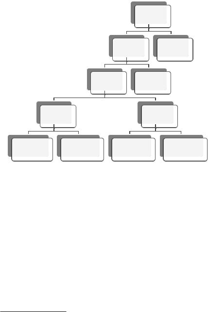
30 |
A. Antimiani et al. |
Baseline 2012
|
|
|
|
|
|
|
All countries |
|
|
|
|
|
|
|
|
||
|
|
|
|
Annex I |
(ET-GLOB) |
|||
|
|
|
|
|
|
|
|
|
|
Emission |
|
No Emission |
|||||
|
|
|||||||
|
|
|||||||
|
Trading |
|
Trading |
|
||||
|
|
(ET) |
|
|
(No-ET) |
|
||
|
|
|
|
|
|
|
||
CBT based on |
|
|
CBT based on |
|||||
domestic |
|
|
|
tariffs ad |
||||
carbon price |
|
|
|
valorem |
||||
|
|
|
|
|
||||
Carbon content |
Carbon content |
Tariffs based on |
Tariffs based on |
|||||
of Annex I |
of Non-Annex |
carbon leakage |
import/output |
|||||
(ET-BAT) |
(ET-BAT) |
rate (ET-CL) |
ratio (ET-IO) |
|||||
Fig. 2.1 Simulation design
The results show that emission trading is a more efficient policy instrument in terms of compliance and welfare costs both for abating countries and at global level. For this reason, we use the corresponding scenario (ET) as a benchmark for the assessment of simulations with trade adjustment policies (Fig. 2.1 ).
Our scenarios are based on ‘one-way’ CBTs applied by abating countries to all imported goods from non-abating countries.4 Since, in GTAP-E, the carbon tax is levied on all energy products consumed in a country, both produced domestically and abroad, the carbon tariff is not applied to imported energy products.
CBTs extend the carbon tax to imports and are established in specific terms, i.e. price per ton of emissions associated with the production of each good. CBT scenarios (ET-NBAT and ET-BAT) are based on a single price for carbon emission resulting from the emission trading, but border taxes are going to differ by sector according to the carbon contents (Bordoff 2009). In the ET-NBAT scenario, border taxes are based on the carbon content of imported goods whereas in the ET-BAT scenario, they are based on the carbon content of the corresponding domestic
4 Border tax adjustments are two-way when they also apply to products exported to non-Annex countries and equal the difference in indirect taxes (e.g. the value added tax) between trading partners. However, this would provide incentives to keep ‘dirty’ plants operating for export purposes and would make meeting the abatement commitments even more difficult for the other firms (Fischer and Fox 2009).

2 Carbon Leakage and Trade Adjustment Policies |
31 |
production in the importing country according to a BAT approach. In the latter case, all non-Annex countries face the same border tax on their exports to each Annex I country, whereas in the former case, all Annex I countries adopt the same policy implying different taxes for the same good according to the country of origin.
The ET-NBAT scenario is likely to be deemed inconsistent with WTO provisions since it discriminates between non-Annex countries as well as between domestic and imported products that are going to face different carbon taxes. The ET-BAT scenario avoids these discriminations, and it is certainly much more realistic in terms of information requirements. Nevertheless, it should be noted that the ad valorem equivalent of the carbon tariff depends on the import price, and this provides an obvious incentive for quality upgrading (Hummels and Skiba 2004).5
By comparing the performance of these two approaches for CBT implementation in terms of efficiency and effectiveness in reducing carbon leakage, we join a large and quickly growing literature. The most innovative part of this chapter elaborates additional scenarios where carbon tariffs are endogenous. The starting point of these scenarios is a given goal, either in terms of carbon leakage rate or competitiveness. The model is then used to compute the sector-specific ad valorem tariffs that would allow the goal to be reached.6
The first counterfactual scenario (ET-CL) is aimed at eliminating carbon leakage. Results show that this goal is unfeasible: even by introducing prohibitive tariffs, only a tiny share of overall non-Annex I emissions is affected, namely, the one resulting from export production. In the model, as well as in reality, emissions result from the choices of different agents whereas exports only concern firms. No tariff can intervene on the drop in energy prices caused by a decrease in the energy demand of Annex I countries, avoiding the corresponding increase in non-Annex demand.
The second counterfactual scenario (ET-IO) is focused on preserving competitiveness. Annex I countries introduce ad valorem tariffs so that the share of imports from non-Annex in total production in each sector of Annex I remains constant. This scenario setting reflects one of the possible interpretations of competitiveness, and other indicators may be adopted.
All the above simulations have been conceived in a non-cooperative setting where Annex I countries adopt unilateral policies in order to cope with the fact that other countries do not act to keep their emissions under control. The final scenario (ET-GLOB)7 simulates a cooperative solution where non-Annex countries agree not to allow their emissions to increase above the 2012 baseline. This would solve the leakage problem by definition, and the introduction of emission trading at world level would represent the most efficient way of reaching emission reduction objectives.
5CBTs are established in specific terms (i.e. price per ton of emissions associated with the production of each good), and their ad valorem equivalents will be higher for goods with lower prices.
6In all simulated scenarios, the tariff surcharges are levied on top of the existing tariff structure by Annex I countries on all imports from the non-Annex countries.
7This scenario can be defined as our first best scenario in contrast with the others which can be referred to as ‘second best’ scenarios.
32 |
A. Antimiani et al. |
2.4Empirical Results
We first compare the implementation of the abatement targets with and without an emission trading scheme (ET and NO-ET scenarios). Simulation results reveal that, when emission trading is allowed, there is a substantial reallocation in emission reductions. The three sellers are the EU, FSU and Belarus. All the other countries buy emission permits. The EU behaviour is hardly surprising if we consider that the new 12 member states are characterized by substantially lower marginal abatement costs and less stringent abatement constraints. The combination of these two elements explains why it is more convenient for the EU as a whole to reduce emissions below the target and sell emission permits in the international market. In line with the expected higher allocative efficiency of market-based instruments, larger abatement efforts are associated with countries with lower marginal abatement costs. As a consequence, the average domestic carbon tax level in the NO-ET scenario ($39.16 per tCO2) turns out to be much higher than the equilibrium price for emission permits in the ET scenario ($22.92 per tCO2).
Both simulations generate carbon leakage, although in the ET scenario, the leakage rate is higher than in the no trade scenario. This result can be explained by considering that the same overall emission reduction objective for Annex I countries is reached with a different abatement allocation in the two scenarios. In the ET scenario, some large economies with demanding abatement targets should implement less structural adjustments and undergo a smaller contraction, thus showing higher imports from non-compliant countries than in the NO-ET scenario. At country level, the non-Annex countries most responsible for carbon leakage in absolute terms are represented by South Africa, Rest of Europe and energyexporting countries and – to a lesser extent – Brazil, India and China.
In terms of welfare effects, there are large discrepancies between the NO-ET and ET scenarios. For net buyers of carbon permits, in the ET scenario, there is a substantial reduction in the allocative efficiency loss since energy-intensive sectors do not have to reduce their production. In other words, the high costs associated with heavy structural adjustments in the production specialization pattern can be avoided. The countervailing effect for net buyers is the expenditure for acquiring permits on the international emission trading market. On the contrary, the emission trading revenue compensates, at least partially, net sellers for the larger adjustments they undergo.
From here on, we consider the emission trading scheme scenario as a reference scenario since its compliance and welfare costs are smaller than those associated with the domestic carbon tax scenario, even if it is not likely to materialize in the near future. Moreover, since the leakage effect is larger, the endogenous carbon tariffs will constitute an upper bound for the implementation of trade adjustment measures aimed at reducing carbon leakage or maintaining competitiveness. In Fig. 2.2, we show the sectoral changes in the leakage rate and self-sufficiency (share of import on sectoral supply) for the Annex I countries as a whole compared with the baseline. As we expect, for coal, gas and energy-intensive sectors, the
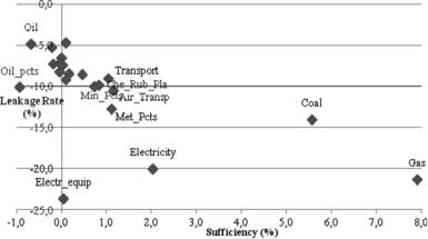
2 Carbon Leakage and Trade Adjustment Policies |
33 |
Fig. 2.2 Leakage rate and sufficiency for Annex I countries in ET scenario (compared with 2012 baseline)
share of import on total output increases due to domestic efforts to comply with the Kyoto Protocol.
Focusing on two major players such as the EU and the USA (Fig. 2.3 ), most sectors show a reduction in domestic production compensated by a surge in imports from non-abating countries. Results for this scenario clearly show the relocation of production from Annex I to non-Annex countries, highlighting the link between environmental policies and competitiveness effects.
Let us now start to analyse the non-cooperative solutions to carbon leakage, according to which an Annex I country adopts unilateral trade adjustment policies. Following Fig. 2.1 , we first compare the two scenarios, ET-NBAT and ET-BAT, simulating exogenous carbon tariffs based on permits equilibrium price. According to our results, the introduction of a CBT is welfare improving for compliant countries with respect to the reference case. In particular, CBTs improve the terms of trade for Annex I countries. By contrast, non-Annex countries register a welfare loss. The welfare improvement in Annex I countries is higher in the ETNBAT scenario where the carbon content used to define the carbon tariff is related to the exporting countries (and for this reason, tariffs are higher than in ET-BAT).
The allocation of emission reductions across Annex I countries hardly changes by applying an exogenous CBT. By contrast, the introduction of tariffs affects emissions from non-Annex countries. In particular, the ET-NBAT scenario reveals a larger impact in terms of leakage reduction, especially for energy exporters, China, India and South Africa. In any case, the environmental effectiveness of these unilateral policies seems to be rather small since, although carbon leakage is uniformly reduced across all non-Annex countries, the overall change is trivial (especially in the ET-BAT scenario). This result can be explained by looking at the share of emissions related to exports by non-Annex towards Annex I countries. If we compare the amount of emissions associated with exports for each non-Annex
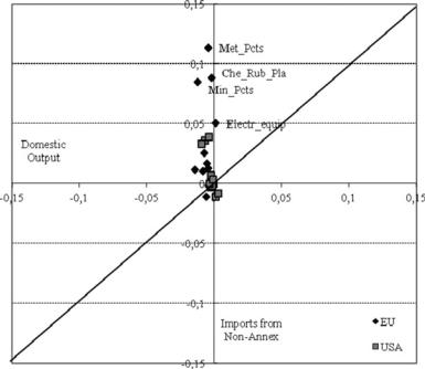
34 |
A. Antimiani et al. |
Fig. 2.3 The EU and US changes in domestic output and imports from non-Annex countries in ET scenario (compared with 2012 baseline)
countries to the Annex I group in the ET scenario with the total amount of emissions produced by firms in non-abating countries, the share of emissions influenced by the CBT is rather low and is even lower if we compare it with total non-Annex emissions. Accordingly, CBTs result in a pure redistribution of unilateral climate change policies costs, without substantial gains in environmental terms.
For the EU and the USA, the two most affected Annex I countries (representative also of seller and buyer behaviours), we then relate changes in domestic output to changes in imports from non-Annex countries maintaining the ET scenario as the baseline. The EU and US domestic production is hardly affected by the CBT when the domestic carbon content is considered (ET-BAT). On the other hand, both countries’ outputs take advantage of the larger import reductions due to the higher tariffs when the carbon content of non-Annex countries is considered (ET-NBAT), especially in energy-intensive sectors (Fig. 2.4).
In the second set of scenarios, carbon tariffs are endogenously determined in order to keep the CO2 emissions of all economic sectors (excluding households) in nonAnnex countries (scenario ET-CL) and the share of imports in total production in Annex I countries (scenario ET-IO) unchanged. In both scenarios, the allocation of emission reduction in Annex I countries is not affected. The ET-CL scenario guarantees the lowest rate of carbon leakage among non-cooperative scenarios, although it is only halved since, for the reasons explained in Sect. 2.3, it cannot be
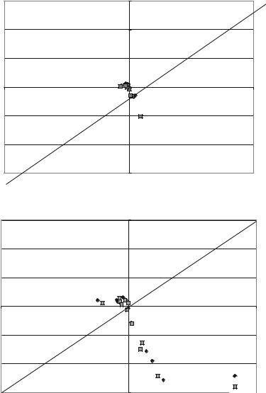
2 Carbon Leakage and Trade Adjustment Policies |
35 |
ET-BTA
0.15
0.1
0.05
Domestic
Output
0 |
-0.05 |
0 |
0.05 |
Che_Rub_Pla 

 Min_Pcts
-0.05
Min_Pcts
-0.1
 EU
EU

 USA
USA
-0.15
Imports from Non-Annex
ET-NBTA
|
0.15 |
|
|
|
0.1 |
|
|
|
0.05 |
|
|
|
Domestic Output |
|
|
-0.05 |
0 |
|
0.05 |
0 |
|
||
|
-0.05 |
|
|
|
Met_Pcts |
|
|
|
Che_Rub_Pla |
Met_Pcts |
|
|
-0.1 |
Che_Rub_Pla |
|
|
|
|
|
|
Min_Pcts |
Min_Pcts |
EU |
|
USA |
||
|
-0.15 |
|
|
|
|
|
Imports from Non-Annex
Fig. 2.4 The EU and US changes in domestic output and imports from non-Annex countries in ET-BAT and ET-NBAT scenarios
eliminated. In particular, some countries, such as China, India, South Africa and Rest of Europe, substantially reduce their emissions, and the contraction of their industrial sector is associated with high welfare losses. In this respect, the higher tariffs of this scenario also lead to very large terms of trade gains for Annex I countries.
36 |
A. Antimiani et al. |
On the other hand, the ET-IO scenario leads to emissions reduction in non-Annex countries which is similar to the outcome of the exogenous CBTs scenarios. The same is true for welfare impacts.
Looking at the relationship between output and import changes in the EU and the USA, Fig. 2.5 shows that the ET-CL scenario features larger reductions than the ET scenario not only for imports but also for domestic supply. It is also worth noting that in the ET-IO scenario, imports only decrease (with respect to the ET scenario) for some energy-intensive sectors and even increase in other cases, especially in the EU market.
If we compare the ad valorem carbon tariffs for alternative scenarios (Table 2.1), it is worth noting that tariffs needed to significantly reduce the carbon leakage problem (ET-CL scenario) are much higher than those currently discussed in the political debate (ET-BAT and ET-NBAT scenarios). It is interesting to note that carbon tariffs aimed at keeping the share of imports from non-Annex countries constant are higher in the energy-intensive sectors. The carbon tariffs in ET-IO scenario – even if not explicitly focused on carbon leakage – imply similar results to the exogenous tariffs based on the carbon content. With regard to non-Annex countries, ET-NBAT and ET-CL scenarios are characterized by higher changes in all sectors which explain their larger welfare costs.
From the Annex I countries point of view, in Table 2.2, we compare changes in the revealed comparative advantage (RCA) index (Balassa 1965) implied by the four different scenarios.
An interesting pattern emerges: the lowest protection scenario (ET-BAT) turns out to be the most effective in improving export competitiveness since it is associated with the highest number of positive RCA changes, meaning that competitiveness compared with the rest of the world is increasing in as many sectors as the number of RCA changes. This confirms that levying high tariffs on manufacturing goods which are intensively used as intermediates in domestic production has a significant negative impact on production costs and consequently on competitiveness.
Finally, we simulate a cooperative scenario in order to obtain a benchmark for comparison with the other results (Table 2.3). In the cooperative scenario, the carbon leakage problem is solved by definition since non-Annex countries are committed to keeping their emissions constant in relation to the 2012 baseline. Moreover, in this scenario, we also observe a much higher global emission reduction since all countries participate in emission trading and non-Annex countries have lower abatement costs. Looking at welfare changes for the world as a whole, our results clearly show that global welfare decreases when CBTs are introduced, as is to be expected, due to the negative impacts on allocative efficiency.
The cooperative scenario would constitute the best solution since welfare changes are more than halved compared with the scenario with emission trading (ET) and almost five times smaller than the scenario designed to partially eliminate carbon leakage through unilateral policies (ET-CL). By looking at the permits equilibrium price, we can shed some light on CBT effects. All scenarios featuring CBTs lead to an increase, albeit rather small, in the price of permits. CBTs protect
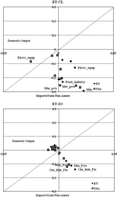
2 Carbon Leakage and Trade Adjustment Policies |
37 |
Fig. 2.5 The EU and US changes in domestic output and imports from non-Annex countries in ET-CL and ET-IO scenario

38 |
|
|
A. Antimiani et al. |
|
Table 2.1 Ad valorem carbon tariffs for alternative scenarios |
|
|
||
|
|
|
|
|
|
ET-BAT |
ET-NBAT |
ET-CL |
ET-IO |
|
|
|
|
|
Agriculture |
1.11 |
1.15 |
21.42 |
0.36 |
Chem., rubb., plast. |
0.71 |
2.15 |
14.47 |
3.32 |
Metal products |
0.62 |
1.97 |
14.40 |
2.10 |
Mineral products |
1.87 |
5.13 |
19.42 |
4.79 |
Oil products |
1.03 |
2.90 |
8.12 |
8.78 |
Paper products |
0.38 |
1.10 |
10.68 |
0.98 |
Average energy-intensive sectors |
0.92 |
2.65 |
13.42 |
3.99 |
Electrical equipment |
0.04 |
0.12 |
9.60 |
0.37 |
Food industry |
0.23 |
0.33 |
14.30 |
0.16 |
Machinery equipment |
0.07 |
0.29 |
12.54 |
0.52 |
Motor vehiclesa |
0.05 |
0.11 |
11.14 |
0.14 |
Other manufacturing |
0.08 |
0.69 |
8.27 |
0.33 |
Textile and leather |
0.14 |
0.41 |
8.81 |
0.33 |
Transport equipment |
0.06 |
0.28 |
12.80 |
0.21 |
Average other sectors |
0.10 |
0.32 |
11.07 |
0.25 |
Total average |
0.49 |
1.28 |
12.77 |
1.70 |
aIn the ET-IO, no CBT are requested for this sector in order to comply with the condition of the scenario
Table 2.2 Changes in RCA for the EU and the USA in alternative scenarios
|
EU |
|
|
|
|
USA |
|
|
|
|
ET- |
ET- |
ET- |
ET- |
ET- |
ET- |
ET- |
ET- |
|
|
BAT |
NBAT |
CL |
IO |
BAT |
NBAT |
CL |
IO |
|
Agriculture |
0.12 |
0.01 |
0.12 |
0.01 |
0.20 |
0.15 |
0.70 |
0.06 |
|
Oil products |
0.09 |
0.12 |
0.03 |
0.09 |
0.11 |
0.03 |
0.07 |
0.01 |
|
Mineral products |
0.13 |
0.11 |
0.10 |
0.12 |
0.08 |
0.02 |
0.02 |
0.02 |
|
Chem., rubb., plast. |
0.41 |
0.25 |
0.10 |
0.21 |
0.11 |
0.01 |
0.09 |
0.02 |
|
Electrical equipment |
0.01 |
0.01 |
0.01 |
0.01 |
0.36 |
0.05 |
0.05 |
0.04 |
|
Transport equipment |
0.07 |
0.12 |
0.02 |
0.10 |
0.79 |
0.13 |
0.54 |
0.16 |
|
Machinery equipment |
0.01 |
0.06 |
0.14 |
0.05 |
0.17 |
0.12 |
0.36 |
0.13 |
|
Motor vehicles |
0.12 |
0.07 |
0.14 |
0.06 |
0.30 |
0.02 |
0.03 |
0.02 |
|
Metal products |
0.23 |
0.09 |
0.11 |
0.10 |
0.01 |
0.01 |
0.03 |
0.02 |
|
Food industry |
0.05 |
0.11 |
0.01 |
0.11 |
0.02 |
0.02 |
0.00 |
0.02 |
|
Paper products |
0.08 |
0,01 |
0.01 |
0.01 |
0.05 |
0.01 |
0.01 |
0.01 |
|
Textile and leather |
0.02 |
0.04 |
0.02 |
0.03 |
0.07 |
0.01 |
0.01 |
0.01 |
|
Other manufacturing |
0.02 |
0.04 |
0.03 |
0.03 |
0.01 |
0.01 |
0.00 |
0.01 |
|
Number of sectors with positive |
10 |
5 |
7 |
5 |
|
9 |
7 |
7 |
7 |
RCA changes respect with |
|
|
|
|
|
|
|
|
|
KT scenario |
|
|
|
|
|
|
|
|
|
|
|
|
|
|
|
|
|
|
|
the domestic production of carbon-intensive sectors which increases the cost of reaching a given overall abatement target, resulting in larger welfare losses.
Table 2.4 shows the impacts of the carbon tax resulting from the global emission trading on energy product prices in selected sectors and countries. Impacts in nonAnnex countries are higher than in Annex I countries since in this scenario, the first
2 Carbon Leakage and Trade Adjustment Policies |
|
|
39 |
||
Table 2.3 Comparing results with a cooperative solution |
|
|
|
||
|
|
|
|
|
|
|
ET-BAT |
ET-NBAT |
ET-CL |
ET-IO |
ET-GLOB |
|
|
|
|
|
|
CO2 reduction (%) |
5.70 |
5.82 |
6.09 |
5.80 |
6.54 |
Leakage rate (%) |
12.91 |
11.09 |
6.95 |
11.43 |
0.00 |
CO2 permits price (US$ per ton |
23.15 |
23.31 |
24.60 |
23.17 |
8.44 |
of CO2) |
54.235 |
55.435 |
100.617 |
56.074 |
20.952 |
Welfare change (million of US$) |
|||||
Table 2.4 Carbon tax average price impacts in selected countries with a cooperative solution
|
|
|
|
|
Rest of |
|
|
Energy |
Rest of |
|
EU |
USA |
Japan |
FSU |
Annex I |
China |
India |
exporters |
non-Annex |
|
|
|
|
|
|
|
|
|
|
Agriculture |
49.78 |
19.59 |
12.82 |
32.78 |
16.90 |
34.29 |
58.35 |
66.49 |
26.33 |
Chem., rubb., plast. |
22.64 |
21.32 |
19.51 |
27.27 |
19.24 |
42.92 |
28.23 |
27.68 |
22.61 |
Electricity |
23.79 |
24.88 |
19.48 |
33.40 |
24.40 |
39.50 |
35.69 |
34.57 |
27.37 |
Metal products |
35.86 |
22.71 |
19.46 |
32.98 |
22.94 |
45.75 |
31.95 |
32.81 |
25.93 |
Mineral products |
26.44 |
22.42 |
19.21 |
32.22 |
23.76 |
46.43 |
32.77 |
31.37 |
25.43 |
Oil products |
17.13 |
9.98 |
0.29 |
29.12 |
15.43 |
73.45 |
14.68 |
21.29 |
18.09 |
Paper products |
28.89 |
21.55 |
39.49 |
34.28 |
21.20 |
49.56 |
31.99 |
31.55 |
27.58 |
Electrical equipment |
72.79 |
24.02 |
24.89 |
38.18 |
24.33 |
75.91 |
37.93 |
55.05 |
31.35 |
Food industry |
30.60 |
22.82 |
16.86 |
35.87 |
22.78 |
47.78 |
38.82 |
32.34 |
28.36 |
Machinery equipment |
31.05 |
22.63 |
17.61 |
35.29 |
21.32 |
53.69 |
41.98 |
17.42 |
24.90 |
Motor vehicles |
34.20 |
23.46 |
26.07 |
34.74 |
21.76 |
59.50 |
41.92 |
33.07 |
26.92 |
Textile and leather |
31.17 |
21.63 |
14.04 |
35.23 |
20.36 |
51.33 |
32.15 |
32.69 |
24.95 |
Transport equipment |
27.93 |
23.71 |
29.23 |
32.86 |
24.04 |
32.23 |
40.53 |
29.97 |
25.07 |
Other manufacturing |
56.62 |
22.72 |
29.07 |
35.09 |
23.93 |
45.51 |
32.96 |
31.80 |
27.48 |
Average |
34.92 |
21.68 |
20.57 |
33.52 |
21.60 |
49.85 |
35.71 |
34.15 |
25.88 |
|
|
|
|
|
|
|
|
|
|
group of countries accounts for a large share of emission reductions. Industrial sectors in China are subject to the highest increase in prices. The impacts of emission trading on prices are relatively high also in the EU and FSU, the Annex I countries in which the greater emission reductions take place.
The distribution of welfare changes in the cooperative scenario reveals that Annex I countries significantly reduce their allocative efficiency losses compared with the ET scenario. The price for this positive pattern is the cost of the emission permits that Annex I countries need to buy on the market. Non-Annex countries face opposite effects since they lose in terms of allocative efficiency, but as net sellers, they gain revenue from the permits sold. More importantly, allocative efficiency gains for Annex I countries are much larger than the allocative efficiency losses for non-Annex countries (Table 2.5). At country level, not all non-Annex countries will gain from participating in a global solution where big gainers are China and energy exporters and big losers are India and Rest of Europe.

Table 2.5 Distribution of welfare impacts in a cooperative solution
|
ET |
|
|
|
ET-GLOB |
|
|
|
|
Permits |
Allocative |
Terms of |
Total welfare |
Permits |
Allocative |
Terms of |
Total welfare |
|
revenue |
efficiency |
trade |
change |
revenue |
efficiency |
trade |
change |
Australia |
1.147 |
1.834 |
1.026 |
4.151 |
822 |
458 |
1.313 |
2.694 |
Belarus |
152 |
528 |
373 |
1.085 |
21 |
232 |
195 |
462 |
Canada |
1.873 |
2.487 |
984 |
5.391 |
1.088 |
612 |
362 |
2.193 |
Croatia |
8 |
75 |
49 |
23 |
12 |
0 |
21 |
20 |
EU |
5.197 |
17.243 |
11.639 |
683 |
228 |
1.989 |
5.800 |
3.194 |
FSU |
9.755 |
7.735 |
3.036 |
1.806 |
1.377 |
2.071 |
2.544 |
2.097 |
Japan |
985 |
4.159 |
5.322 |
387 |
976 |
305 |
4.489 |
2.475 |
New Zealand |
155 |
115 |
72 |
205 |
77 |
24 |
26 |
90 |
Norway |
289 |
289 |
2.707 |
2.876 |
126 |
72 |
1.486 |
1.574 |
Swiss |
3 |
422 |
399 |
203 |
40 |
84 |
270 |
20 |
USA |
10.521 |
20.937 |
6.545 |
25.089 |
8.592 |
5.193 |
3.627 |
9.527 |
Annex I |
124 |
54.769 |
16.650 |
36.118 |
10.563 |
10.575 |
8.723 |
12.044 |
Brazil |
0 |
237 |
355 |
344 |
109 |
254 |
558 |
289 |
China |
0 |
149 |
1.885 |
14 |
6.081 |
2.994 |
1.446 |
3.840 |
India |
0 |
697 |
1.014 |
1.854 |
1.196 |
1.413 |
1.242 |
838 |
Mexico |
0 |
960 |
1.482 |
2.496 |
130 |
1.703 |
657 |
2.292 |
South Africa |
0 |
97 |
2 |
78 |
803 |
488 |
36 |
348 |
ENEEXP |
0 |
305 |
22.484 |
21.969 |
1.461 |
2.347 |
16.763 |
16.299 |
Rest of Africa |
0 |
4 |
258 |
171 |
56 |
126 |
184 |
209 |
Rest of America |
0 |
104 |
348 |
359 |
120 |
253 |
519 |
319 |
Rest of Asia |
0 |
1.205 |
3.572 |
3.851 |
515 |
564 |
4.621 |
3.874 |
Rest of Europe |
0 |
403 |
232 |
829 |
117 |
211 |
403 |
385 |
Non-Annex |
0 |
1.325 |
16.817 |
17.334 |
10.587 |
10.354 |
8.779 |
8.908 |
Total |
124 |
53.445 |
167 |
53.452 |
24 |
20.929 |
56 |
20.952 |
|
|
|
|
|
|
|
|
|
40
.al et Antimiani .A
2 Carbon Leakage and Trade Adjustment Policies |
41 |
2.5Conclusions
In this chapter, we propose alternative border tax adjustments for dealing with carbon leakage. We simulate different scenarios to gain a better understanding of to what extent a border tax is effective in reducing the leakage rate and if major differences emerge when alternative CBTs are modelled. More specifically, we are interested in investigating the impact in terms of leakage reduction and to what extent such trade policies are also a valid instrument for protecting the economic competitiveness of compliant countries in the international market.
From our results, we can affirm that the effectiveness of CBTs in reducing carbon leakage is limited and that they could even be damaging in terms of competitiveness when CBTs act on prices of goods produced by non-abating countries and are used as intermediates in abating countries. Moreover, border tariff adjustment feasibility with respect to WTO rules is a moot point, and justifying them with climate concerns could open the way to a proliferation of highly distortive unilateral measures.
When comparing CBT effectiveness with a global cooperative scenario, our results clearly suggest that a cooperative solution would be highly preferable both in terms of welfare impacts and allocative efficiency in emission reduction. In fact, the cooperative solution is welfare improving with respect to all CBT forms. This last point suggests that the bargaining power exerted by Annex I countries in the post-Kyoto agreement should be directed towards a global solution including major emerging economies in the policymaking process rather than towards unilateral solutions in which a domestically oriented point of view prevails.
Acknowledgements The authors wish to thank Giancarlo Tosato and Maria Rosa Virdis for their comments and suggestions. This work has been supported by the research network Enea- Inea-Uniroma Tre on Integrating bottom-up and top-down energy models: the case of GTAP-E and Markal TIMES-Italy.
References
Atkinson, G., Hamilton, K., Ruta, G., & Van der Mensbrugghe, D. (2010). Trade in ‘Virtual Carbon’: Empirical results and implications for policy (World Bank Policy Research Working Paper Series 5194). Washington, DC: The World Bank.
Balassa, B. (1965). Trade liberalization and revealed comparative advantage. The Manchester School of Economic and Social Studies, 33, 92–123.
Bordoff, J. (2009). International trade law and the economics of climate policy: Evaluating the legality and effectiveness of proposals to address competitiveness and leakage concerns. In L. Brainard & I. Sorkin (Eds.), Climate change, trade, and competitiveness: Is a collision inevitable (Brookings trade forum 2008/2009). Washington, DC: The Brookings Institution.
Burniaux, J., & Oliveira, M. (2000). Carbon emission leakages: A general equilibrium view
(OECD Economics Department Working Papers, No. 242). Paris: OECD.
Burniaux, J. M., & Truong, T. (2002). GTAP-E: An energy-environmental version of the GTAP model (GTAP Technical paper N 16). mimeo.
42 |
A. Antimiani et al. |
Copeland, B. R., & Taylor, M. S. (2004). Trade, growth, and the environment. Journal of Economic Literature, 21, 7–71.
Dong, Y., & Whalley, J. (2008). Carbon, trade policy, and carbon free trade areas (NBER Working Paper No. 14431). Cambridge: NBER.
Dong, Y., & Whalley, J. (2009). How large are the impacts of carbon motivated border tax adjustments (NBER Working Paper No. 15613). Cambridge: NBER.
Energy Modeling Forum. (2000, February 23–25). EMF 18 model comparisons. Stanford: Energy Modeling Forum.
Felder, S., & Rutherford, T. F. (1993). Unilateral CO2 reductions and carbon leakage: The consequences of international trade in oil and basic materials. Journal of Environmental Economics and Management, 25, 162–176.
Fischer, C., & Fox, A. K. (2009). Comparing policies to combat emissions leakage (Discussion Paper 09-02). Washington, DC: Resources for the Future.
Gerlagh, R., & Kuik, O. J. (2007). Carbon leakage with international technology spillovers
(FEEM Working Paper No. 33). Milan: FEEM.
Haaparanta, P., Kerkela¨, L., Liski, M., Riipinen, T., & Sulamaa, P. (2001). Climate change policies, world markets, and Finland (Working Paper). Helsinki: Helsinki School of Economics.
Hamasaki, H. (2007). Carbon leakage and a post-Kyoto framework (Research Paper No.287). Japan: Fujitsu Research Institute.
Hummels, D., & Skiba, A. (2004). Shipping the good apples out? An empirical confirmation of the Alchian–Allen conjecture. Journal of Political Economy, 112, 1384–1402.
Kuik, O. J. (2001, June 27–29). The effect of trade liberalization on carbon leakage under the Kyoto protocol: Experiments with GTAP-E. Paper prepared for the 4th annual conference on global economic analysis. West Lafayette: Purdue University.
Kuik, O. J., & Verbruggen, H. (2002). The Kyoto regime, changing patterns of international trade and carbon leakage. In L. Marsaliani, M. Rauscher, & C. Withagen (Eds.), Environmental economics and international economy (pp. 239–257). Dordrecht: Kluwer Academic Publishers.
Mattoo, A., Subramanian, A., van der Mensbrugghe, D., & He, J. (2009). Reconciling climate change and trade policy (WP 09-15). Washington, DC: Peterson Institute for International Economics.
McDougall, R., & Golub, A. (2007). GTAP-E release 6: A revised energy-environmental version of the GTAP model (GTAP Technical Paper No. 15). mimeo.
McKibbin, W. J., Ross, M. T., Shackleton, R., & Wilcoxen, P. J. (1999). Emissions trading, capital flows and the Kyoto protocol (Economics and Environment Network Working Papers 9901). Australian National University, Economics and Environment Network.
Moore, O. M. (2010). Implementing carbon tariffs. A fool’s errand? (World Bank Policy Research Working Paper Series 5359). Washington, DC: The World Bank.
OECD. (2003). Environmental policy in the steel industry: Using economic instruments. Paris: OECD.
OECD. (2005). The competitiveness impact of CO2 emissions reduction in the cement sector. Paris: OECD.
OECD. (2006). The political economy of environmentally related taxes. Paris: OECD. Schenker, O., & Bucher, R. (2010). On interactions of optimal climate policy and international
trade. An assessment of border carbon measures. University of Bern and Oeschger Center for climate change, Munich Personal RePEc Archive.
Stern, N. (2006). The economics of climate change – The stern review. Cambridge: Cambridge University Press.
Veenendaal, P., & Manders, T. (2008). Border tax adjustment and the EU-ETS, a quantitative assessment (CPB Document No. 171). The Hague: Central Planning Bureau.
Wang, S., De Groot, H. L. F., Nijkamp, P., & Verhoef, E. T. (2009). Global and regional impacts of the clean mechanism (Tinbergen Institute Discussion Paper 09-045/3). The Netherlands.
2 Carbon Leakage and Trade Adjustment Policies |
43 |
Wooders, P., & Cosbey, A. (2010). Climate-linked tariffs and subsidies: Economics aspects (competitiveness & leakage). IISD, Thinking Ahead on International Trade (TAIT) – 2nd Conference climate change, trade and competitiveness: Issues for the WTO, Geneva: The Graduate Institute, Center for Trade and Economic Integration.
World Bank. (2010). State and Trends of the Carbon Market 2010. Carbon Finance at the World Bank, Environment Department. Washington, DC: The World Bank.

Chapter 3
Theoretical Approaches to Dynamic Efficiency in Policy Contexts: The Case of Renewable Electricity
Pablo Del Rı´o and Mercedes Bleda
Abstract Dynamic efficiency (or the ability of a policy instrument to generate a continuous incentive for technical improvements and cost reductions in technologies) is central to the assessment and choice of environmental and energy policies in long-run scenarios where innovation lock-in is relevant. This is also the case in instruments that support electricity from renewable energy sources (RES-E). In contrast with effectiveness and static efficiency assessment criteria, the innovation effects of such support have received much less attention from both a theoretical and an empirical perspective. Several theoretical perspectives have paid some attention to these innovation effects, including the traditional economics approach, the systems of innovation perspective and the literature on learning effects. The aims of this chapter are to provide an overview of those perspectives and to build bridges between them.
Keywords Renewable electricity • Dynamic efficiency • Innovation lock-in
• Energy policy • Systems of innovation
The work in this paper has been supported by a mobility grant awarded by the Spanish Ministry of Science and Innovation to Mercedes Bleda as a visiting Research Fellow at the CCHS, CSIC.
P. Del Rı´o (*)
Institute for Public Goods and Policies (IPP), Centro de Ciencias Humanas y Sociales,
Consejo Superior de Investigaciones Cientı´ficas (CSIC), C/Albasanz 26-28, Madrid 28037, Spain
Institute for Public Goods and Policies (IPP), Consejo Superior de Investigaciones Cientı´ficas (CSIC), Serrano 117, Madrid 28006, Spain
e-mail: pablo.delrio@csic.es
M. Bleda
Institute for Public Goods and Policies (IPP), Centro de Ciencias Humanas y Sociales,
Consejo Superior de Investigaciones Cientı´ficas (CSIC), C/Albasanz 26-28, Madrid 28037, Spain
Manchester Institute of Innovation Research (MIoIR), Manchester Business School, University of Manchester, Harold Hankins Building, Manchester, Booth Street West, Manchester M13 9PL, UK
e-mail: mercedes.bleda@mbs.ac.uk
V. Costantini and M. Mazzanti (eds.), The Dynamics of Environmental |
45 |
and Economic Systems: Innovation, Environmental Policy and Competitiveness,
DOI 10.1007/978-94-007-5089-0_3, # Springer Science+Business Media Dordrecht 2013

46 |
P. Del Rı´o and M. Bleda |
3.1Introduction
The world faces pressing challenges arising from the energy sector, including the provision of increased quantities of affordable energy needed to meet economic aspirations, limiting the economic vulnerabilities of oil dependence and reducing CO2 emissions from fossil-fuel burning. Improving energy-supply technologies in general and renewable energy technologies in particular is a prerequisite for surmounting these challenges in a timely and cost-effective way. It is now widely acknowledged or recognised that technological advance has the potential to significantly decrease the costs of attaining societal goals such as climate change mitigation (Newell 2010).
The criterion of dynamic efficiency is central to the assessment and choice of environmental and energy policies in long-run horizons where innovation lock-in is relevant. This is also the case with instruments that support electricity from renewable energy sources (RES-E). Dynamic efficiency is understood as the capacity of a policy instrument to induce a continuous incentive for technological improvements and cost reductions in existing renewable energy technologies, facilitate the advancement of emerging technologies along the technological change pipeline and promote the diffusion of renewable energy technologies with different maturity levels.
In contrast to effectiveness and static efficiency assessment criteria, the innovation effects of this support have received much less attention from both a theoretical and an empirical perspective. Several theoretical perspectives have paid some attention to these innovation effects, including the traditional economics approach, the systems of innovation perspective and the literature on learning effects. The aims of this chapter are to provide an overview of those perspectives and to build bridges between them.
The dynamic efficiency of environmental policy instruments in general, and RES-E support schemes in particular, is a very relevant topic. Kneese and Schulze (1975) pointed out early that, besides the issue of static efficiency, the extent to which policy instruments spur new technology towards the efficient conservation of the environment is one of the most important criteria on which to judge the performance of environmental policy instruments (Requate 2005).1
The relative importance of the dynamic effects of alternative policy instruments on technological change (and hence long-term compliance costs) is greater in environmental problems which are of great magnitude and/or have very long time horizons. Hence, the increased attention given by scholars and policymakers to
1 However, some authors are doubtful about the relative importance of dynamic efficiency criteria compared with more traditional, static efficiency criteria. For example, Parry et al. (2003) stress that the welfare gain from innovation is sometimes not much greater than the welfare gain of efficiently abating pollutants by means of conventional technologies. Requate (2005) observes that resources to engage in R&D are scarce. Hence, environmental technological progress may crowd out other strands of welfare enhancing technological progress. Finally, Fischer and Newell (2008) argue that the underlying process of technological change turns out to be far less important than the incentives to use technology efficiently to reduce emissions.

3 Theoretical Approaches to Dynamic Efficiency in Policy Contexts. . . |
47 |
the problem of global climate change has greatly increased the prominence of the dynamic efficiency of environmental and energy policy instruments, including RES-E support schemes (Jaffe et al. 2002). Given the ambitious targets in the RES realm everywhere (EU, USA and China), a great deal of focus has been placed on the role of innovation in lowering the costs of these non-emitting energy sources (Fischer and Newell 2008).
RES-E support schemes refer to policies aimed at encouraging the diffusion of renewable electricity technologies. Three main types of RES-E support schemes are usually considered: feed-in tariffs, quotas with tradable green certificates (TGCs) and tendering/bidding procedures. These are usually complemented with secondary instruments, including investment subsidies and fiscal incentives (del Rı´o and Gual 2004).
3.2Theoretical Approaches to Analysis of Innovation Effects of RES-E Support
The innovation effects of RES-E support can be analysed from several perspectives.
3.2.1The Traditional Economics Perspective2
Several theoretical approaches, including mainstream environmental economics, are based on the linear model of innovation which states that technologies go through sequential stages without major interactions between them. In the environmental economics literature (Jaffe et al. 2002; Requate 2005; del Rı´o 2009), innovation is regarded as a black box—into which R&D inputs flow and out of which commercial technologies diffuse into the marketplace—to the detriment of the intermediary role for supply and demand interactions (Taylor 2008). The effects on the different stages of innovation are analysed separately, disregarding the interactions between stages (Popp 2010). Assuming perfect economic rationality, decisions are based on microeconomic optimisation behaviour, triggered by price changes. The treatment of technological change is either exogenous or assumed to respond automatically to changes in relative prices as a result of exogenous developments (such as environmental or energy policies).
In turn, embracing the linear model of innovation involves the recommendation of policies based on R&D and commercialisation strategies, seeing the problem essentially in terms of a low level of R&D or carbon prices in the energy sector.
2 Following Marechal (2007), we use the word traditional to avoid the problems arising from the somewhat ambiguous use of the term neoclassical. Traditional economics refers to the Walrasian model of welfare economics, which can be defined as the theoretical synthesis of the Marshallian approach with marginal production theory (Marechal 2007).
48 |
P. Del Rı´o and M. Bleda |
It is assumed that technologies, once created, are optimally deployed in response to whatever policy incentives may or may not be in place (Popp 2010). The main argument derives from the theory of induced innovation (Hicks 1932): changing relative prices induce innovations. Since the hypothesis is that the rate and direction of innovation are likely to respond to changes in relative prices, changing costs for energy use (e.g. through the implementation of environmental or energy policies) are assumed to lead to incentives for future inventions and innovations (Jaffe et al. 2002; Walz and Schleich 2009; Requate 2005).
Contributions within this tradition normally analyse the cost-efficiency of RES- E deployment and support instruments by comparing them with CO2 mitigation instruments (Palmer and Burtraw 2005; Fischer and Newell 2008). Indeed, there is a tendency in this literature to undermine the relevance of RES-E support schemes. The existence of a double externality is acknowledged: an environmental and a technological one. The former is internalised through a CO2 price and the latter through public R&D support (Newell 2008; Jaffe et al. 2005). No RES-E policy is as cost-effective as a cap-and-trade policy for achieving carbon emission reductions (Palmer and Burtraw 2005; Fischer and Newell 2008). However, the time horizon considered is usually too short, and the mitigation targets are modest. This plays against capital-intensive technologies (with a large cost-reduction potential), such as renewables (IEA 2008). The framework adopted is usually static, disregarding dynamics and the interdependencies between institutions, actors and technologies in complex systems leading to inertia and lock-in. Furthermore, competitive pressure is regarded as the main (or exclusive) mechanism to reduce the costs of technologies, disregarding other dimensions of dynamic efficiency such as diversity. Generally, technology-neutral instruments are advocated.
3.2.2The Systems of Innovation Perspective
The systems of innovation (SI) approach (Carlsson et al. 2002) stresses that innovations are not developed and implemented in isolation but within a technological and sociocultural context. It focuses on the importance and interdependencies of actors, networks, institutions, cumulative learning processes and spatial and technological characteristics (Edquist 2005). It adopts a holistic perspective and considers phenomena such as path dependency, lock-in, interdependence, nonlinearity and co-evolution (Edquist 2005; Markard and Truffer 2008). This approach can reveal how innovation occurs in relation to particular technologies, industrial sectors and specific national contexts, what system failures may be occurring and how innovation may be influenced by incentives and policies (Foxon and Andersen 2009).
Following Unruh (2000, p. 819), technological systems are defined as “interrelated components connected in a network or infrastructure that includes physical, social and informational elements”. An innovation system consists of three elements (Malerba 2004; Woolthuis et al. 2005): technology and related knowledge

3 Theoretical Approaches to Dynamic Efficiency in Policy Contexts. . . |
49 |
and skills, networks of actors and institutions. Networks of actors develop and implement new knowledge and technology within their institutional context. For an innovation system to be successful in developing and implementing technologies, these three building blocks, which co-evolve in time, need to be aligned.
This approach has already been applied to analyse renewable energy systems (Astrand and Neij 2006; Jacobsson and Bergek 2004; Foxon et al. 2005; Jacobsson 2008; Walz and Schleich 2009, among others). These papers stress that a shift towards renewable energy technology systems is a complex process which involves changes in the aforementioned elements of an innovation system. They identify the system failures related to the development, commercialisation and diffusion of renewable energy technologies.
This perspective tries to cope with some of the drawbacks of the conventional perspective which has been much criticised for its conceptualisation of technological change. The systemic approach provides corrections to this criticism and suggests policy implications that are different from (although not necessarily contradictory to) those derived from the conventional approach:
•Feedback between stages. In particular, innovation and diffusion are not sequential phases, but learning and future innovations depend on experiences made during market diffusion. That is, the creation of a market for renewable technologies feeds back into investments in R&D.
•Path dependency and lock-in. One drawback of studies based on environmental economics is the fact that they do not look at system changes and interdependencies, although such system changes are necessary to reach longterm emission reduction goals (Rogge and Hoffmann 2010). In contrast, the systemic perspective acknowledges that barriers to renewable energy are systemic (also termed system failures; see Nill and Kemp 2009). These systemic barriers lead to lock-in through a path-dependent process driven by technological and institutional internal returns to scale.
Technologies are not only linked to other technologies but are also interrelated with the cultural and institutional aspects of their environment (Marechal 2007). Carbon lock-in has been used to denominate the persistent dominance of highcarbon technologies (in spite of the existence of low-carbon ones).3 Unruh (2000, p. 817) defines carbon lock-in as the “interlocking technological, institutional and social forces that can create policy inertia towards the mitigation of global climate change”. This lock-in occurs through a “path-dependent process driven by technological and institutional increasing returns to scale”. Dynamic economies of scale and learning effects are a major source of lock-in. R&D investments and diffusion
3 A stream of the economic literature on climate change mitigation has applied an evolutionary approach with the aim of emphasising the inertia in current technological systems (Kemp 1996; Unruh 2000, 2002; Marechal 2007; del Rı´o and Unruh 2007; Rip and Kemp 1998; Foxon et al. 2005).
50 |
P. Del Rı´o and M. Bleda |
provide a source of improvement and cost reductions for existing technologies. The later effect takes place because diffusion allows technologies to benefit from learning effects and dynamic economies of scale. Emerging, more expensive, technologies may fall into a vicious circle: they are not adopted because they are too expensive, and they are too expensive because they are not adopted.
Barriers to technological change are multifaceted, and the price factor is only one of the factors affecting technological changes. Technological change is endogenous to an economic system in which there are both inducement and blocking mechanisms. Changes in relative prices are only one of the inducement mechanisms. In addition to demand and technology factors, this approach underlines the importance of several factors (characteristics of innovation, actors, networks and institutions, including regulations) (Suurs and Hekkert 2009). These factors influence each other, highlighting the importance of feedback mechanisms and cumulative causation processes. Therefore, price signals are necessary albeit not sufficient to encourage innovation in new technological systems.
The implication for RES-E policy is that the inducement mechanisms need to be strong enough to overcome these interrelated barriers to RES-E and set a process of cumulative causation in motion that works in favour of the new technology.
Lately, the SI approach has been further developed following several avenues, namely, by trying to integrate it with the multilevel approach of technological transitions (Geels and Schot 2007), as done by Markard and Truffer (2008), and by identifying the functions of an innovation system (Hekkert and Negro 2009; Bergek et al. 2008).4 With regard to this last point, different innovation systems can be assessed and compared in terms of the functions they fulfil in order to derive policy recommendations to support the development of a specific technology (Hekkert et al. 2007; Negro et al. 2007). Functions are emergent properties of the interplay between actors and institutions (Markard and Truffer 2008). The function approach identifies those properties in a technological innovation system that are needed in order to introduce sustainable energy technologies successfully (Hekkert and Negro 2009).
Cumulative causation suggests that system functions may reinforce each other over time, thereby resulting in a virtuous cycle (Hekkert et al. 2007; Jacobsson and Bergek 2004). The diffusion of renewable energy technologies into the incumbent energy system requires virtuous circles to be established between the different functions (Suurs and Hekkert 2009; Hekkert and Negro 2009). Similarly, Jacobsson and Johnson (2000) argue that there are three central issues for the emergence of a new technological system based on renewable energy technologies: variety in the knowledge base increased by experimentation, institutional change aligned to the needs of renewable energy technology and the emergence of strong actors who can promote the new technology.
4 Assessment in terms of system functions is one of the main approaches of the systems of innovation literature. Other innovation system studies have placed more emphasis on structural analyses (Carlsson et al. 2002; Jacobsson and Johnson 2000). Currently, some authors are concentrating on the integration of both approaches (Markard and Truffer 2008).

3 Theoretical Approaches to Dynamic Efficiency in Policy Contexts. . . |
51 |
Such interactions may take place in a niche which can be created by public policy through, for example, RES-E support instruments. Niches allow technologies to progress and create a supportive institutional environment around it. Once they do so, technologies become a technological regime, as is the case for wind energy in many European countries. The SI approach points to the importance of policy interventions that support all system elements—technology and cost development as well as actor involvement—for introduction and deployment of renewable energy technologies.
The coalition of forces/actors and the cumulative causation process have not been stressed by the traditional approach but both are particularly relevant in the RES-E support realm. Although actors are embedded in an institutional context, they may also deliberately change or adapt existing institutions or create new ones (Edquist and Johnson 1997). Radical innovations are often promoted by actor networks that show little overlap with prevailing actor structures in a sector or technological field (Markard and Truffer 2008). In turn, once a coalition of forces has been formed, it is likely to organise the lobbying of changes in public support, which feeds back into the deployment of the technology. For example, wind power actors, together with biogas stakeholders, have been shown to lobby in favour of better feed-in payment conditions for renewable energy technologies (Markard et al. 2009). A coalition of forces results from the sequential interaction between support, market creation, stages of technological change and actors (Markard et al. 2009).5
The forming of markets is therefore a necessary requirement for setting a learning process in motion. Stimulating RES-E will create virtuous cycles between actors and stages of technological change, providing further investment opportunities and expanding the market for key technologies (Lee et al. 2009). This suggests the importance of implementing policies that result in cumulative causation processes leading to an effective deployment of RES-E in a long-term perspective.
Only public policy may break lock-in. However, not all policies are equally useful in encouraging the emergence of new technologies. The systems of innovation approach stresses the difficulties that a new technology, such as renewables, faces when penetrating a market and competing with a dominant technology which has benefited from economies of scale and learning effects and from the adaptation of the institutional environment to the existing technology. In order for renewable energy technologies to develop, the forces of inertia that prevail in the incumbent energy system have to be broken. We argue that different RES-E support instruments and design elements can exert significant influences on the direction of technological development a technological system takes.
Nevertheless, since the systemic perspective emphasises the wide array of barriers to RES-E, it suggests that deployment policies are only one of the factors (although a crucial one) that encourage RES-E. When this perspective has been
5 For example, in his analysis of wind energy deployment and policy in Denmark, Spain and Sweden, Meyer (2007) provides empirical evidence of the role of the coalition of forces in encouraging wind energy in Spain.

52 |
P. Del Rı´o and M. Bleda |
applied to RES-E support, several barriers have been shown to constrain RES-E.6 Given the complexity of stages and drivers influencing technological change, it is unlikely that a single policy instrument would be sufficient to trigger major technological changes. Smits and Kuhlmann (2004) argue that system innovation processes require systemic instruments, that is, those that support system functions. Since RES-E support instruments cannot tackle all functions, they are not systemic instruments, although they can be made part of systemic policy packages.
In spite of the usefulness of this approach, there is a relative paucity of studies using it. Walz and Schleich (2009) review the empirical literature on RES-E support schemes and conclude that “these studies, by and large, do not analyse the effects on innovation within an integrated systems of innovation view”.
3.2.3The Literature on Learning Effects
A recent albeit abundant literature has stressed the role of learning effects in reducing the costs of technologies in general and renewable energy technologies in particular. However, this literature is not isolated from what was mentioned above since many energy-economy models that incorporate induced technological change include some learning effects and the literature on systems of innovation stresses the importance of these effects.
The specialised literature on learning emphasises two main components of technical change and energy costs: cumulative research, development and demonstration (RD&D) and cumulative installed capacity or learning-by-doing (see Sagar and van der Zwaan 2006; IEA 2008; Kahouli-Brahmi 2008). Whereas certain components of cost improve with R&D investment, others are likely to respond to increased deployment of the technology (Nemet and Baker 2010).
Learning assumes that a technology’s performance improves as experience with the technology accumulates. Learning is an aggregate term that may involve a number of different mechanisms that all contribute to cost reduction over time when producing and deploying new technologies. This chapter focuses on those learning effects that are dynamic and have direct innovation effects:
•Learning-by-doing (Arrow 1962) refers to the repetitious manufacturing of a product leads to improvements in the production process.
•Learning-by-using (Rosenberg 1982) refers to improvements in the technologies as a result of feedback from user experiences of the innovation process.
•Learning-by-interacting (Lundvall and Johnson 1994) takes place as a result of network interactions between actors.
6 The assessment of Astrand and Neij (2006) shows that early inflexible steering of technology and market development, together with a lack of comprehensive, long-term strategy, lack of continuity in policy interventions and weak combinations of policy programmes and measures, have contributed to very limited wind power development in Sweden.

3 Theoretical Approaches to Dynamic Efficiency in Policy Contexts. . . |
53 |
Often, combinations of these factors occur in each stage of the market diffusion process and the contribution of each changes over time. The importance of those learning effects varies along the technological change pipeline and for different technologies.7 In turn, each cost element (material costs, process costs and overhead costs) is affected by different mechanisms as empirically shown by Kalowekamo and Baker (2009).
Cost reductions have been assessed through learning curves.8 In learning curves, the experience gained with a certain technology is expressed as a learning rate (percentage at which the unit cost decreases with every doubling of cumulative installed production).9
These learning effects have been incorporated into energy-economy models (Kahouli-Brahmi 2008). A key message from these models is that policy needs explicitly to consider the learning potential associated with investments and accelerate abatement in order to induce cost reductions. Endogenisation of technological learning induces early investments in initially expensive technologies since future revenues offset the short-run additional investments (Kahouli-Brahmi 2008).
The extent to which instruments and design elements are able to encourage those learning effects is a main aspect of RES-E support. Obviously, learning effects only take place when deployment is increased, suggesting that there is a clear synergy between the effectiveness of a RES-E support instrument and learning effects. For socio-technical systems like the wind power system, where an important barrier to market introduction and expansion is high investment costs, policy instruments should support and accelerate the learning process (Astrand and Neij 2006).
3.3Combining Different Perspectives: Points of Complementarity and Conflict
All of the approaches have their limitations, and all are approximations that miss some important phenomena underlying the complex nature of technological change, with important effects on the results of RES-E policy. For example, although the traditional economics perspective provides the seminal economic theory for the analysis of the innovation effects of environmental regulation, the approach disregards fundamental system changes and technology-related
7For example, Junginger et al. (2006) show that for technologies developed on a local level (e.g. biogas plants), learning-by-using and learning-by-interacting are important learning mechanisms whereas for CHP plants utilising fluidised bed boilers, upscaling is probably one of the main mechanisms behind cost reductions. Nemet and Baker (2010) show that certain components of the costs of solar PV improved with R&D investment, whereas others responded to increased deployment of the technology.
8Some authors have stressed the difficulties in building learning curves for some renewable energy technologies (Junginger et al. 2006) or criticised the learning curve model itself (Kahouli-Brahmi 2008).
9For a recent analysis of (observed) learning rates for various electricity supply technologies, see IEA (2008) and Kahouli-Brahmi (2008), among others.

54 |
P. Del Rı´o and M. Bleda |
interdependencies that are necessary to reach long-term emission reduction goals (Rogge and Hoffmann 2010). The energy-related SI studies do not analyse the specific impact of environmental regulations on the innovation system; they downplay the role of competition as a source of cost reductions and technological improvements and have sometimes been criticised for not generating sufficient practical policy advice (Bergek et al. 2008; Rogge and Hoffmann 2010; Woolthuis et al. 2005). We therefore regard the aforementioned perspectives as complementary in the analysis of the dynamic efficiency of RES-E support schemes. Therefore, they should be combined in order to include all the relevant innovation effects resulting from RES-E promotion.
Thus, a combined framework may offer benefits that, for the task of analysing dynamic efficiency, go beyond the merits of each approach. In this section, we sketch the main foundations of such integration which should be improved and fully detailed in future research. Our aim is to briefly summarise a number of conceptual issues a combined framework should strive to address and the links and bridges between the different outlined approaches.
In particular, a combined approach will be highly beneficial if it meets some or all of the aspects identified as shortcomings in one of the frameworks. In order not to become overly complex or create overlaps, this framework should clarify the relevance, need and application domain of each of its conceptual elements (Markard and Truffer 2008). The integration is spurred on by two interrelated requirements: the need to broaden analytical perspectives in order to take all the relevant dimensions of dynamic efficiency into account and the need to provide lessons to promote RES-E in a dynamically efficient manner by considering those dimensions. We believe that bridges could be built between the approaches.10 Other authors have also called for a broadening of the analytical framing regarding the set of considerations used to explain the emergence and success of innovation (Walz and Schleich 2009).
Of course, major points of disagreement exist between those approaches, but two are worth highlighting: (1) technological diversity vs. technological competition and (2) linear vs. systemic perspective of (renewable) technological change. While the conventional approach emphasises competition between technologies, the systems of innovation approach stresses the relevance of the diversity of innovations, learning effects from deployment and feedbacks from deployment to R&D. The systemic approach suggests that significant feedback loops between stages, actors and key variables may exist and that cumulative causation is crucial. In contrast, competition between innovators as a source of cost reductions and improvements in the technologies has been downplayed by the systems of innovation approach in the analysis of the barriers to RES-E deployment. While some insights or hypotheses from the traditional approach are compatible with the systemic approach (i.e. technological competition), others are certainly incompatible (i.e. the linear approach to technological change).
We propose that this integration be built on a systems of innovation approach since it provides a broader and richer picture of the innovation process in renewable
10 The literature seems to be too polarised in this respect, with theoretical and empirical studies following either one or the other approach. Exceptions are Rogge and Hoffmann (2010) and Walz and Schleich (2009).

3 Theoretical Approaches to Dynamic Efficiency in Policy Contexts. . . |
55 |
energy than the conventional environmental economics approach and, thus, offers a guiding heuristic on how the RES-E support policies may influence this process.
The systemic approach could easily integrate the insights from the learning literature (all learning effects). Indeed, bridges between them are inherent and/or have been explicitly built. Innovation and learning are typically activities that take place in systems (Lundvall 1992). Technological learning can be regarded as the process in which actors acquire knowledge in order to improve the performance of the technological system (Smits and Kuhlmann 2004). As Smits and Kuhlmann (2004) point out, an innovation system covers the actors who produce knowledge on the supply side, the actors who implement innovation on the demand side, as well as the actors who link supply and demand plus the actors who support the entire system. To pinpoint what is going on in the technological system, we need to describe the learning processes for all these actors precisely as well as the interaction between these learning processes.
Learning effects show two explicit points of connection with the SI approach: the interrelationships between stages and the interactions between the institutional and the technological realms.11
With regard to the former, Sagar and van der Zwaan (2006) note that the different forms of learning often also feedback into the technology R&D process, leading to improved technologies and products in the future. Whereas typically R&D precedes deployment, it may be advantageous to undertake them simultaneously or iteratively, so as to exploit the possible interaction between them (Sagar and van der Zwaan 2006).
As far as the second point is concerned, the presumption is that each element in the innovation system (the technology, the actors, the institutions and the cost of technology) needs to be part of the development and deployment process which could be characterised as a learning process. The learning process is essential for all elements of the system (Astrand and Neij 2006).
Learning may lead to systemic improvements, an example of which would be the institutional evolution that allows the lowering of costs in projects in which new technologies are used (Sagar and van der Zwaan 2006). This suggests a relationship between learning, R&D and institutional changes, with feedback loops between them.12
11Indeed, learning effects introduce nonlinearities and positive feedbacks into the models in which they are used (the more a technology is used, the greater the incentive for using it more) (McDonald and Schrattenholzer 2001).
12Watanabe et al. (2000) convincingly showed that the political environment behind Japanese government support for PV innovation was critical in developing the interindustry partnerships basic public research and broad-based market promotion for this fledging industry which in turn led to and was a result of learning effects. The authors analysed the Japanese solar PV Sunshine Project which aimed to encourage the broad involvement of cross-sectoral industry, stimulate inter-technology stimulation and cross-sectoral technology spillover and induce vigorous industry investment in PV R&D, leading to an increase in industry’s PV technology knowledge stock. They showed that an increase in this technology knowledge stock contributed to a dramatic increase in solar cell production. These increases led to a dramatic decrease in solar cell production price, and this decrease induced a further increase in solar cell production. An increase in solar cell production induced further PV R&D, thus creating a “virtuous cycle” between R&D, market growth, learning effects and price reduction.

56 |
P. Del Rı´o and M. Bleda |
Learning-by-interacting establishes an explicit link between learning and the systems approach. Smit et al. (2007) show that learning-by-interacting is crucial to achieving the necessary binding elements in the technology-specific innovation system. During the diffusion of the technology, the network interactions between actors such as research institutes, industry, end users and policymakers generally improve (Lundvall 1988; Junginger et al. 2006). The relationship between diffusion and learning goes in both directions: while learning-by-interacting allows the firm to benefit from external sources of learning and is greatly associated with the increasing diffusion of technology (Kahouli-Brahmi 2008), the interactions between the various actors including the research laboratories, the industry, the end users and the political decision-makers enhance the diffusion of knowledge (Lundvall 1988).
Since learning-by-interacting can take place intentionally via collaboration or through the creation of niches, there is a role for public policy in stimulating the interaction between different actors. The actors from the industrial part of the technological system should get better access to actors in academia and other actors (Smit et al. 2007).13 Astrand and Neij (2006) empirically showed how the introduction of subsidies in the early 1990s in Sweden increased the diversity of actors involved in the development process of wind turbines and how the involvement of additional actors improved the learning in using wind turbines. The literature on Strategic Niche Management has also argued that whether or not a change of technological regime comes about depends, among other factors, on the occurrence of learning processes within protected spaces (or niches). Through experimentation and learning in niches (and/or between the niches and regime level), innovative ideas and technologies may mature and become better suited to change or replace the until then dominant regime (Van Mierlo et al. 2010).
Nevertheless, consideration of learning effects does not involve the adoption of an SI approach, although every systemic approach has to include those effects. For example, although some energy-economy models now incorporate a form of learning processes with increasing returns (see Ko¨hler et al. 2006), they do not include the main features of the SI approach, namely, systemic interdependencies, heterogeneity of agents (as a result of bounded rationality) and historical contingencies (Marechal 2007).
Regarding the link between Sections 3.2.1 and 3.2.3, learning effects can be regarded as a market failure in the sense of the traditional approach. As argued by Jaffe et al. (2002), the presence of increasing returns in the form of learning effects suggests that market outcomes for technologies exhibiting these features may be inefficient.
13 For example, in the analysis of the Dutch wind-offshore sector, Smit et al. (2007) argued that there was weak learning-by-interacting by the actors from the industrial part of the technology system, who should get better access to actors in academia and actors in the oil and gas industry. The authors showed that there were several barriers hindering this interaction process. In contrast, they also showed that in the Danish case, learning-by-interacting occurred between knowledge institutes, component suppliers, project operators and turbine manufacturers and Danish policies contributed to the formation of these interactions.
3 Theoretical Approaches to Dynamic Efficiency in Policy Contexts. . . |
57 |
However, the combination of Sections 3.2.1 and 3.2.2 is more difficult although the systems approach, and the traditional approach may be compatible on different time frames. As argued by Faber and Frenken (2009), the policy implications that can be drawn from innovation system studies are more long term and, consequently, often rather impressionistic. As such, insights from these studies are complementary to neoclassical policy insights that apply well to well-defined, short-term problems.
Regarding the combination between Sections 3.2.2 and 3.2.3, Gru¨bler et al. (1999) already noted that, since technological learning is a classical example of increasing returns (i.e. the more learning takes place, the better a technology’s performance), the mathematical solutions are non-convex (the more investment, the lower the costs), which would be especially difficult to handle in traditional optimisation models and algorithms. However, the modelling literature on endogenous technical change related to low-carbon technologies has proved that learning effects can be introduced in traditional models without much friction (see Edenhofer et al. 2009). The insights of the conventional approach (notably, the dynamic efficiency resulting from technological competition) may/should be incorporated into a broader integrated conceptual framework. This links to the literature on RES-E support schemes which has traditionally stressed the relevance of competition between actors, particularly between equipment suppliers and RES-E generators leading to cost reductions in the technologies. This vision of dynamic efficiency is useful, although certainly not sufficient, and should be included in the integrated approach. This vision has been understated in the SI approach. This add-on is certainly not incompatible with the SI approach. Competition between those actors would be an aspect of the broader relationship between different elements of the innovation system and between those actors, institutions and RES-E support policy in particular.
3.4Conclusions
Technological change is a complex process with different stages and barriers and drivers for each stage. The sources of technological change are also diverse, and there are several strands of thought regarding the determinants of innovative activity. Thus, the analysis of the capacity of RES-E support instruments to encourage technological changes should take this diversity into account. The dynamic efficiency of RES-E support instruments can indeed be analysed with several perspectives. This suggests that several dynamic factors are at play, that dynamic efficiency is in fact a multilayered criterion and that those different layers should be made explicit (Verbruggen 2009).
This chapter has discussed relevant approaches to the analysis of the dynamic efficiency of environmental and energy instruments and, particularly, RES-E support schemes. It has aimed to provide the first steps of an integration of approaches by building bridges between them. This is deemed highly useful in order to structure the realisation of empirical studies on the dynamic efficiency of RES-E support. An obvious avenue for further research is therefore advance in the
58 |
P. Del Rı´o and M. Bleda |
integration of approaches. Furthermore, the few case studies that deal with energy issues with a systems of innovation approach have not analysed the implications of different RES-E support instruments and different design elements. This lack of consideration of the design elements is also a limitation of the conventional environmental economics approach. There is therefore a clear need to integrate research on the specific effects of RES-E design into a wider system of innovation approach (Walz and Schleich 2009). Therefore, a comparative analysis of different RES-E support schemes according to the complementary dimensions derived from those approaches is worth undertaking.
References
Arrow, K. J. (1962). The economic implications of learning by doing. Review of Economic Studies, 29, 155–173.
Astrand, K., & Neij, L. (2006). An assessment of governmental wind power programmes in Sweden—using a systems approach. Energy Policy, 34, 277–296.
Bergek, A., Jacobsson, S., Carlsson, B., Lindmark, S., & Rickne, A. (2008). Analyzing the functional dynamics of technological innovation systems – A scheme of analysis. Research Policy, 37(3), 407–429.
Carlsson, B., Jacobsson, S., Holmen, M., & Rickne, A. (2002). Innovation systems: Analytical and methodological issues. Research Policy, 31(2), 233–245.
Del Rı´o, P. (2009). The empirical analysis of the determinants for environmental technological change: A research agenda. Ecological Economics, 68(3), 861–878.
Del Rı´o, P., & Gual, M. (2004). The promotion of green electricity in Europe: Present and future.
European Environment Journal, 14, 219–234.
Del Rı´o, P., & Unruh, G. (2007). Overcoming the lock-out of renewable energy technologies in Spain: The cases of wind and solar electricity. Renewable and Sustainable Energy Review, 11(7), 1498–1513.
Edenhofer, O., Carraro C., Hourcade J.-C., Neuhoff K., Luderer G., Flachsland C., Jakob M., Popp A., Steckel J., Strohschein J., Bauer N., Brunner S., Leimbach M., Lotze-Campen H., Bosetti V., de Cian E., Tavoni M., Sassi O., Waisman H., Crassous-Doerfler R., Monjon S., Dro¨ge S., van Essen H., del Rı´o P., Tu¨rk A. et al. (Ed.) (2009). The Economics of decarbonization (Report of the RECIPE Project). Potsdam: Potsdam-Institute for Climate Impact Research.
Edquist, C. (2005). Systems of innovation: Perspectives and challenges. In J. Fagerberg, D. Mowery, & R. Nelson (Eds.), Oxford handbook of innovation (pp. 181–208). Oxford: Oxford University Press.
Edquist, C., & Johnson, B. (1997). Institutions and organisations in systems of innovation. In C. Edquist (Ed.), Systems of innovation: Technologies, institutions and organizations. London/ Washington: Pinter/Cassell Academic.
Faber, A., & Frenken, K. (2009). Models in evolutionary economics and environmental policy: Towards an evolutionary environmental economics. Technological Forecasting and Social Change, 76, 462–470.
Fischer, C., & Newell, R. (2008). Environmental and technology policies for climate mitigation.
Journal of Environmental Economics and Management, 55(2), 142–162.
Foxon, T., & Andersen, M. (2009). The greening of innovation systems for eco-innovation – Towards an evolutionary climate mitigation policy. Paper presented at the Summer DRUID Conference, Copenhagen Business School.
3 Theoretical Approaches to Dynamic Efficiency in Policy Contexts. . . |
59 |
Foxon, T., Gross, R., Chase, A., Howes, J., Arnall, A., & Anderson, D. (2005). U.K. Innovation systems for new and renewable energy technologies: Drivers, barriers and systems failures.
Energy Policy, 33, 2123–2137.
Geels, F., & Schot, J. (2007). Typology of sociotechnical transition pathways. Research Policy, 36, 399–417.
Gru¨bler, A., Nakicenovic, N., & Victor, D. (1999). Dynamics of energy technologies and global change. Energy Policy, 27(5), 247–280.
Hekkert, M., & Negro, S. (2009). Functions of innovation systems as a framework to understand sustainable technological change: Empirical evidence from earlier claims. Technological Forecasting and Social Change, 76, 584–594.
Hekkert, M., Suurs, R., Negro, S., Kuhlmann, S., & Smits, R. (2007). Functions of innovation systems: A new approach for analysing technological change. Technological Forecasting and Social Change, 74, 413–432.
Hicks, J. (1932). The theory of wages. London: Macmillan. IEA. (2008). Energy technology perspectives. Paris: IEA.
Jacobsson, S. (2008). The emergence and troubled growth of a ‘biopower’ innovation system in Sweden. Energy Policy, 36, 1491–1508.
Jacobsson, S., & Bergek, A. (2004). Transforming the energy sector: The evolution of technology systems in renewable energy technology. Industrial and Corporate Change, 13(5), 815–849.
Jacobsson, S., & Johnson, A. (2000). The diffusion of renewable energy technology: An analytical framework and key issues for research. Energy Policy, 28(9), 625–640.
Jaffe, A. B., Newell, R., & Stavins, R. (2002). Environmental policy and technological change.
Environment and Resource Economics, 22(1–2), 41–69.
Jaffe, A. B., Newell, R., & Stavins, R. (2005). A tale of two market failures: Technology and environmental policy. Ecological Economics, 54(2–3), 164–174.
Junginger, M., de Visser, E., Hjort-Gregersen, K., Koornneef, J., Raven, R., Faaij, A., & Turkenburg, W. (2006). Technological learning in bioenergy systems. Energy Policy, 34, 4024–4041.
Kahouli-Brahmi, S. (2008). Technological learning in energy–environment–economy modelling: A survey. Energy Policy, 36, 138–162.
Kalowekamo, J.,& Baker, E. (2009). Estimating the manufacturing cost of purely organic solar cells. Solar Energy, 83(8), 1224–1231.
Kemp, R. (1996). The transition from hydrocarbons: The issues for policy. In S. Faucheux, D. W. Pearce, & J. Proops (Eds.), Models of sustainable development (pp. 151–175). Cheltenham: Edward Elgar.
Kneese, A., & Schulze, C. (1975). Pollution, prices, and public policy. Washington, DC: Brookings Institute.
Ko¨hler, J., Grubb, M., Popp, D., & Edenhofer, O. (2006). The transition to endogenous technical change in climate-economy models: A technical overview to the innovation modelling comparison project. Energy Journal, 27, 17–56.
Lee, B., Lliev, L., & Preston, F. (2009). Who owns our low carbon future? Intellectual property and energy technologies. London: Chatham House Report.
Lundvall, B. (1988). Innovation as an interactive process: From user-producer interaction to the national system of innovation. In G. Dosi et al. (Eds.), Technical change and economic theory. London: Pinter Publishers.
Lundvall, B. (1992). National systems of innovation. London: Printer Publisher.
Lundvall, B., & Johnson, B. (1994). The learning economy. Journal of Industry Studies, 1(2), 23–42. Malerba, F. (2004). Sectoral systems of innovation: Basic concepts. In F. Malerba (Ed.), Sectoral systems of innovation: Concepts, issues and analyses of six major sectors (pp. 9–41).
Cambridge: Cambridge University Press.
Marechal, K. (2007). The economics of climate change and the change for climate in economics.
Energy Policy, 35(10), 5181–5194.
Markard, J., & Truffer, B. (2008). Technological innovation systems and the multi-level perspective: Towards an integrated Framework. Research Policy, 37, 596–615.
Markard, J., Stadelmann, M., & Truffer, B. (2009). Analysis of variation in innovation systems. Identifying potential development options for biogas in Switzerland. Research Policy, 38(4), 655–667.
60 |
P. Del Rı´o and M. Bleda |
McDonald, A., & Schrattenholzer, L. (2001). Learning rates for energy technologies. Energy Policy, 29(4), 255–261.
Meyer, N. (2007). Learning from wind energy policy in the EU: Lessons from Denmark, Sweden and Spain. European Environment, 17, 347–362.
Negro, S., Hekkert, M., & Smits, R. (2007). Explaining the failure of the Dutch innovation system for biomass digestion—A functional analysis. Energy Policy, 35, 925–938.
Nemet, G., & Baker, E. (2010). Demand subsidies versus R&D: Comparing the uncertain impacts of policy on a pre-commercial low-carbon energy technology. The Energy Journal, 30(4), 49–80.
Newell, R. (2008). A U.S. innovation strategy for climate change mitigation (Discussion Paper 2008-15; Hamilton Project). Washington, D.C.: Brookings Institution.
Newell, R. (2010). The role of markets and policies in delivering innovation for climate change mitigation. Oxford Review of Economic Policy, 26(2), 253–269.
Nill, J., & Kemp, R. (2009). Evolutionary approaches for sustainable innovation policies: From niche to paradigm. Research Policy, 38(4), 668–680.
Palmer, K., & Burtraw, D. (2005). Cost-effectiveness of renewable electricity policies. Energy Economics, 27(6), 873–894.
Parry, I., Pizer, W., & Fischer, C. (2003). How large are the welfare gains from technological innovation induced by environmental policies? Journal of Regulatory Economics, 23(3), 237–255.
Popp, D. (2010). Innovation and climate policy (NBER Working Paper 15673). Cambridge: NBER. http://www.nber.org/papers/w15673
Requate, T. (2005). Dynamic incentives by environmental policy instruments—A survey. Ecological Economics, 54, 175–195.
Rip, A., & Kemp, R. (1998). Technological change. In S. Rayner & E. Malone (Eds.), Human choice and climate change (Vol. 2, pp. 327–399). Columbus: Battelle.
Rogge, K., & Hoffmann, V. (2010). The impact of the EU ETS on the sectoral innovation system of power generation technologies – Findings for Germany. Energy Policy, 38, 7639–7652.
Rosenberg, N. (1982). Inside the black box: Technology and economics. Cambridge: Cambridge University Press.
Sagar, A., & van der Zwaan, B. (2006). Technological innovation in the energy sector: R&D, deployment and learning-by-doing. Energy Policy, 34, 2601–2608.
Smit, T., Junginger, M., & Smits, R. (2007). Technological learning in offshore wind energy: Different roles of the government. Energy Policy, 35, 6431–6444.
Smits, R., & Kuhlmann, S. (2004). The rise of systemic instruments in innovation policy.
International Journal of Foresight and Innovation Policy, 1(1), 4–32.
Suurs, R., & Hekkert, M. (2009). Cumulative causation in the formation of a technological innovation system: The case of biofuels in the Netherlands. Technological Forecasting and Social Change, 76, 1003–1020.
Taylor, M. (2008). Beyond technology-push and demand-pull: Lessons from California’s solar policy. Energy Economics, 30, 2829–2854.
Unruh, G. (2000). Understanding carbon lock-in. Energy Policy, 28(12), 817–830. Unruh, G. (2002). Escaping carbon lock-in. Energy Policy, 30, 317–325.
Van Mierlo, B., Leeuwis, C., Smiths, R., & Woolthuis, R. (2010). Learning towards system innovation: Evaluating a systemic instrument. Technological Forecasting and Social Change, 77(2), 318–334.
Verbruggen, A. (2009). Performance evaluation of renewable energy support policies, applied on Flanders’ tradable certificates system. Energy Policy, 37(4), 1385–1394.
Walz, R., & Schleich, J. (2009). The economics of climate change policies: Macroeconomic effects, structural adjustments and technological change. Heidelberg: Physica Verlag, Springer.
Watanabe, C., Wakabayashi, K., & Miyazawa, T. (2000). Industrial dynamism and the creation of a virtuous cycle between R&D, market growth and price reduction. The case of Photovoltaic Power Generation (PV) development in Japan. Technovation, 20(6), 299–312.
Woolthuis, R., Lankhuizen, M., & Gilsing, V. (2005). A system failure framework for innovation policy design. Technovation, 25, 609–661.

Chapter 4
Energy Efficiency Policy in the USA:
The Impact of the Industrial Assessment
Centres (IAC) Programme and State
and Regional Climate Policy Actions
Luis Maria Abadie, Ramon Arigoni Ortiz, Ibon Galarraga, and Anil Markandya
Abstract The impact that two US policies have had on energy consumption and carbon emissions of small and medium enterprises (SME) is analysed in this chapter. The first policy is the Industrial Assessment Centres (IAC) programme from the Department of Energy (DOE) of the US government in which assessments are offered to companies to identify energy efficiency (EE) measures. A probit model is used for a clearer understanding of EE investment determinants in SMEs. The second consists of the US State and Regional Climate Policy actions of the US Environmental Protection Agency (EPA). Panel data is used to analyse the impact of both policies, combining information on emissions and energy consumption per unit of real GDP for 51 US states over 19 years with data on EE investments as a consequence of the first policy, and, finally, 30 climate policies implemented at state and regional levels. The results show that some policies are more effective than others in reducing energy consumption and carbon emissions. There are also notable differences across states regarding climate policy and investment decisions.
Keywords Energy efficiency policy • Regional policy • Small and medium enterprises • Policy effectiveness • Investment decisions
L.M. Abadie • R.A. Ortiz • I. Galarraga (*)
BC3 Basque Centre for Climate Change, Gran Via 35-2, 48009 Bilbao, Spain e-mail: lm.abadie@bc3research.org; ramon.ortiz@bc3research.org; ibon.galarraga@bc3research.org
A. Markandya
Ikerbasque Professor and BC3 Basque Centre for Climate Change, Gran Via 35-2, 48009 Bilbao, Spain
e-mail: anil.markandya@bc3research.org
V. Costantini and M. Mazzanti (eds.), The Dynamics of Environmental |
61 |
and Economic Systems: Innovation, Environmental Policy and Competitiveness,
DOI 10.1007/978-94-007-5089-0_4, # Springer Science+Business Media Dordrecht 2013

62 |
L.M. Abadie et al. |
4.1Introduction
The extraction, transport and consumption of fossil fuels as well as depletion of nonrenewable resources generate significant environmental impacts such as greenhouse gas (GHG) emissions. Low efficiency in the use of this energy source increases energy needs, costs and impacts. This is one of the reasons why energy efficiency (EE) policies, together with an increasing use of renewable energy, are an essential part of climate policies. At the same time, EE policies are a smart way of reducing resource depletion and energy costs, while the benefits of the policy can often exceed investment costs. The typology of applied EE policies includes informationand awareness-raising campaigns as well as different subsidy schemes. These in general can be rapidly implemented and therefore form a good policy option for the short and medium term. EE has been one of the mainstays of energy policy in recent years, be it for reasons of competitiveness in the economy, availability of resources or other reasons of a more strategic, geopolitical nature.
In the manufacturing industry, EE measures play a major role as the sector accounts for nearly a third of the world’s energy consumption: 31% of the world primary energy use and 36% of CO2 emissions (IEA 2007). However, investments that seem to be economically worthwhile are not always made. This phenomenon is known as the energy efficiency paradox (Jaffe et al. 2004; DeCanio 1998; De Groot et al. 2001; Linares and Labandeira 2010; Eichhammer 2004; Patton 2001) and has been explained by insufficient information, principal-agent problems, lack of access to capital and/or divergences between social and private discount rates. While the cost of this typology of investments is known, the future savings and the return of the investment can depend on the weather and/or the production conditions that prevail (Kissock and Eger 2008). This inherent uncertainty significantly reduces the implementation of EE measures as shown in studies by Sandberg and So¨derstro¨m (2003) and De Groot et al. (2001). In many situations, energysaving information can be effectively improved with the use of monitoring and measuring systems where information and communication technologies (ICT) can play a major role in contributing towards reducing uncertainty and increasing the implementation of EE measures. This information is clearly relevant to EE investment decision, and there has been a strong view among policy-makers that it can help promote such investment (see below) (Bunse et al. 2011). Characteristics of the companies that face the investment such as size, number of employees, expected future earnings growth or price to earnings ratio also affect the decisions as shown by DeCanio and Watkins (1998) for the Green Light programme.
As in many other countries, efforts to improve EE have been a core part of energy policy in the USA for many years and several policies have been tried such as the EPA ENERGY STAR labelling programme1 and the so-called Industrial Assessment Centres (IAC) programme of the US Department of Energy’s Office of Energy Efficiency and Renewable Energy.2
1See Boyd et al. (2008) for more information on industrial plant manufacturing energy use.
2For more information, see http://www.iac.rutgers.edu
4 Energy Efficiency Policy in the USA. . . |
63 |
This chapter looks at this second programme which has been underway since 1976, with the aim of getting industry to increase productivity and reduce its environmental impact through energy efficiency, waste minimisation and prevention of atmospheric pollution. The programme is based on EE in-plant assessments performed on site at small and medium enterprises (SME) in the manufacturing sector. The IAC programme aims to reduce the knowledge gap existing among SME managers since this has been identified as an important barrier to EE investments by Thollander and Ottosson (2010) and Rohdin et al. (2007) among others. Bunse et al. (2011) also identify an important gap between the existing EE solutions and the degree of implementation in the industry sector. Of course, companies that are intensive in energy use have a greater propensity to invest in EE, especially when energy prices are high or are expected to increase significantly in the future. The price of emission permits is also a determinant that has been identified.
Several other studies have analysed and used the information contained in the IAC database. For example, Tonn and Martin (2000) look at the changes over time in corporate decision-making on energy efficiency using a seven-stage model; Anderson and Newell (2004) develop a number of logit models calibrated with data from 1981 to 2000 to show positive impacts for shorter payback periods, lower investment cost, greater annual energy savings, increased energy costs and greater energy conservation; Abadie et al. (2010) estimate various decision-making models with data from 1984 to 2008 to identify measures to support investments in electricity-related EE. This study presented here complements previous research in the following ways: (a) data until 2009 is used, (b) state-level variables are introduced for GDP and emissions, (c) dummy variables to account for EPA policies are also included, (d) panel data is used per US state and finally (e) the impact of the IAC programme, state policies and EPA policies on energy consumption and emissions is analysed.
4.2Determinants of Investments in Energy Efficiency
4.2.1Investment Decision: Previous Evidence
A preliminary analysis of the IAC raw data suggests that along with other temporary effects which are difficult to determine there is also, as might be expected, a depletion effect in investment opportunities. In other words, the best investments are made first and less attractive measures are left for later. We observe that the investment implementation rate is relatively low given the total number of recommendations made. This probably indicates that the recommendations made are not as suitable as they could be, that other factors exist that are judged to be more important than these recommendations when it comes to deciding whether or not to invest, or a combination of the two.
There is also clear evidence from econometric models (Anderson and Newell 2004; Abadie et al. 2010) in support of the idea that the payback time variable is

64 |
L.M. Abadie et al. |
determinant in investment decisions, as might be expected. Investment cost is also highly important.
When applying two families of models (payback time and cost/benefit), Abadie et al. (2010) showed that:
1.Changes in payback time have a non-linear influence on investment decisions, and so the tendency is different depending on the time frames involved.
2.The probability that an investment will be made decreases as the payback time
increases, whereas the sensitivity of accepting an investment in the face of variations in payback time is negative and increases with the payback value.3
The lower the payback, a decrease on it generates a greater positive impact in the probability of acceptance.
3.Firms located in the states with the highest levels of GHG emissions are more likely to invest in EE. Furthermore, according to preliminary results, states with more stringent environmental legislation also have higher levels of investment in EE.
4.Firms located in the states where GDP from manufacturing industry is highest are less likely to invest in EE.
5.Up-front investment cost has more influence on investment decisions than potential benefits in the future.
6.Logically, the rate of investment in EE should be highest when considerable savings (or benefits) are expected from low-cost investments, but there is a maximum percentage of 70% of recommendations implemented, which is not easily exceeded even when these two favourable factors are combined.
7.Both reductions in costs and increases in expected savings increase the likelihood of an EE investment project being accepted although the impact of the latter is lower than that of the former.
When it comes to offering recommendations on policy design, the need to study the context in which investments take place in greater depth cannot be obviated; other aspects that must be assessed include behaviour patterns, availability of loans and other financial factors that may influence decisions. Even so, the results presented here offer some useful indicators of important factors that should be useful to policy-makers.
Particularly noteworthy is the importance of payback time compared with other variables, especially in investments with payback times of less than 1 year. The link between this variable and the soundness of the assessment teams may merit a more thorough investigation but lies outside the scope of this study. Therefore, any policy that directly or indirectly helps to reduce payback time must initially be seen as an option worth bearing in mind. As payback time increases, the effectiveness of policies gradually decreases. It can therefore also be stated that measures affecting shorter payback times will be more efficient than those affecting longer payback times. For the latter, more specific, nuanced policies may be preferable.
The GDP of the state where measures are to be implemented is another important variable that must be considered. Perhaps counter intuitively, firms located in
3 See Abadie et al. (2010) for more details on how this is estimated.
4 Energy Efficiency Policy in the USA. . . |
65 |
geographical areas where aggregate output is lower are found to be more likely to invest as a result of the programme. This greater likelihood to accept support among industries in areas with lower sectoral GDP shares may be a clear reflection that such firms are in greater need of support than others whose results are better. Likewise, firms in states where GHG emission levels are highest are found to be more likely to invest as per the recommendations made under the programme. In other words, in terms of both actual needs for support and sensitivity to changes in behaviour as a result of policies, regions with low or sectoral GDPs and higher emission levels should be targeted on a priority basis by public sector policies.
Given that cost seems to outweigh potential benefits as a factor in deciding whether to make an investment, policies that focus on cost should be more effective in getting firms to make investments in energy efficiency. Instruments such as tax deductions, direct subsidies, cheaper loans and taxes on pollution-causing activities seem to be the best options for encouraging energy efficiency in specific areas of activity. Instruments that focus on future savings, such as carbon pricing and energy pricing policies, are likely to be less useful in achieving this objective. This apparent paradox suggests that along with the proven need for worldwide carbon pricing policies (Neuhoff 2008), measures to help reduce the total cost of investment rather than the relative cost continue to be essential, and above all highly effective, in supporting certain industries and sectors. The well-known shorttermism effect (which, as mentioned above, can be seen even among individuals) can also be seen in industrial activities (Graham et al. 2005). A detailed analysis of the actual discount rates applied in these industrial sectors may shed more light on this matter.
Finally, the depletion effect and the apparent existence of an investment ceiling or maximum (found here to be around 70%) suggest that policies of this type should be reassessed regularly to gauge their actual impact and make any adjustments that may be needed to ensure their continued effectiveness.
4.2.2The IAC Database 2011
The information contained in the IAC database (by 03/24/2011) is used in this chapter. These are a total of 14,890 assessments and 111,567 recommendations, that is, an average of 7.49 recommendations per assessment.
The information available was adjusted for the purposes of this study resulting in a total of 101,286 recommendations as follows:
•Records dating from before 1984 to after 2009 are disregarded in order to give a data period of 26 years with full information. The records for 2010 and 2011 were ruled out because the final outcomes of many of the recommendations are not yet known.
•The sample is restricted to decisions reported as implemented and not implemented. This means excluding recommendations whose status is not reported or is pending and those recorded as data excluded or unavailable.

66 |
L.M. Abadie et al. |
•A minor series of 129 records for Puerto Rico has been excluded.
•Additionally, 31 records were also eliminated since no information at state level was available.
Table 4.1 below shows the number of recommendations per state and the rate of implementation. Note that the rate is never higher than 61% or lower than 29%.
Figure 4.1 shows the evolution of the implementation rate with an apparent depletion effect—that is, a fall off in the implementation rate. The relatively low energy prices during the 1990s decade may also explain the significant reduction in the implementation rate for that period. In Fig. 4.2, the implementation rate (represented by the line) and recommendations (represented by bars) are depicted per activity sector (SIC code4). We can clearly see that some sectors are more prone to invest than others with great disparity on the implementations among industries. For instance, the petroleum and coal sector, an energy intensive sector, with few recommendations, has a high rate of implementation. The implementation rate per sector varies from 46.8% in printing and publishing to 54.9% in petroleum and coal.
4.2.3The Decision Concerning Energy Efficiency Investment in the IAC Programme
In order to analyse the investment decisions of the SMEs participating in the IAC programme, two probit models are estimated. The first one, using more recent data and almost double the number of recommendations, including other sources of energy as well as electricity, other efficiency measures such as waste minimisation and pollution prevention and direct productivity enhancements, follows the findings in Abadie et al. (2010) and relates the decision on implementing the recommendation to the payback time as follows:
y ¼ b0 þ b1 lnðpbÞ þ b2 ln ðpbÞ2 þ e |
(4.1) |
where |
|
y ¼ 1 if y > 0 and y ¼ 0 if y 0 |
|
Therefore, |
|
Pr½y ¼ 1& ¼ F b0 þ b1 lnðpbÞ þ b2 ln ðpbÞ2 |
(4.2) |
where F is the normal cumulative distribution function.
The functional form with the quadratic term is used as Abadie et al. (2010) showed a non-linear relationship with the implementation rate.
4 (SIC) The Standard Industrial Classification that represents the principle product manufactured by the plant.
Table 4.1 Recommendations per state and degree of implementation
State |
N recommendations |
% Implementation |
State |
N recommendations |
% Implemented |
Alabama |
966 |
48 |
Nebraska |
893 |
54 |
Alaska |
81 |
58 |
Nevada |
847 |
47 |
Arizona |
3,177 |
41 |
New Hampshire |
689 |
51 |
Arkansas |
2,080 |
59 |
New Jersey |
1,889 |
49 |
California |
7,884 |
48 |
New Mexico |
187 |
42 |
Colorado |
4,096 |
58 |
New York |
2,582 |
51 |
Connecticut |
1,028 |
50 |
North Carolina |
3,489 |
51 |
Delaware |
343 |
41 |
North Dakota |
61 |
43 |
Florida |
4,366 |
45 |
Ohio |
5,714 |
53 |
Georgia |
3,843 |
49 |
Oklahoma |
3,660 |
54 |
Hawaii |
61 |
61 |
Oregon |
2,547 |
55 |
Idaho |
169 |
39 |
Pennsylvania |
3,173 |
49 |
Illinois |
6,151 |
40 |
Rhode Island |
263 |
51 |
Indiana |
2,441 |
42 |
South Carolina |
651 |
48 |
Iowa |
2,641 |
52 |
South Dakota |
254 |
48 |
Kansas |
2,424 |
52 |
Tennessee |
2,716 |
52 |
Kentucky |
1,175 |
43 |
Texas |
6,032 |
60 |
Louisiana |
1,872 |
54 |
Utah |
620 |
29 |
Maine |
1,465 |
52 |
Vermont |
203 |
61 |
Maryland |
452 |
49 |
Virginia |
1,695 |
48 |
Massachusetts |
2,080 |
51 |
Washington |
935 |
51 |
Michigan |
2,596 |
45 |
West Virginia |
1,187 |
57 |
Minnesota |
1,482 |
52 |
Wisconsin |
2,159 |
41 |
Mississippi |
1,933 |
40 |
Wyoming |
138 |
56 |
Missouri |
3,853 |
57 |
Total US states |
101,286 |
50 |
Montana |
43 |
42 |
|
|
|
|
|
|
|
|
|
. . .USA the in Policy Efficiency Energy 4
67
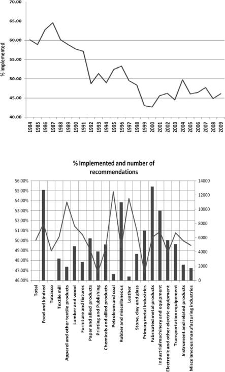
Fig. 4.1 Implementation rate
Fig. 4.2 Implementation rate and recommendations per SIC code
4 Energy Efficiency Policy in the USA. . . |
|
|
|
69 |
||
Table 4.2 Probit analysis of the decision to implement IAC recommendations |
|
|||||
|
|
|
|
|
|
|
Probit regression |
|
|
|
Number of obs ¼ |
85,935 |
|
|
|
|
|
Wald chi2(2) ¼ |
1,614.86 |
|
Log pseudolikelihood ¼ 58,690.38 |
|
Prob > chi2 ¼ |
0.0000 |
|
||
|
Pseudo R2 ¼ |
0.0144 |
|
|||
Implementation |
|
Robust std. |
z |
P>jzj |
[95% Conf. |
|
status |
Coef. |
err. |
|
interval] |
|
|
ln(pb)2 |
0.1476 |
0.0043 |
34.45 |
0.000 |
0.1560 |
0.1392 |
ln(pb) |
0.0137 |
0.0014 |
9.77 |
0.000 |
0.0164 |
0.0109 |
Constant (b0) |
0.0586 |
0.0048 |
12.11 |
0.000 |
0.0681 |
0.0491 |
Table 4.3 Probit analysis of the decision—costs and benefits associated with IAC |
|
|||||
|
|
|
|
|
|
|
Probit regression |
|
|
|
Number of obs ¼ |
86,090 |
|
|
|
|
|
Wald chi2(2) ¼ |
2,445.83 |
|
Log pseudolikelihood ¼ 58,375.483 |
|
Prob > chi2 ¼ |
0.0000 |
|
||
|
Pseudo R2 ¼ |
0.0216 |
|
|||
Implementation |
|
Robust std. |
z |
P>jzj |
[95% conf. |
|
status |
Coef. |
err. |
|
interval] |
|
|
ln(cos) |
0.1361 |
0.0031 |
43.96 |
0.000 |
0.1422 |
0.1301 |
ln(ben) |
0.0571 |
0.0361 |
15.83 |
0.000 |
0.0500 |
0.0642 |
Constant (b0) |
0.5495 |
0.0206 |
26.60 |
0.000 |
0.5090 |
0.5900 |
Results are shown in Table 4.2.
Both the payback time of the investment in energy efficiency and its square are highly significant and negative in sign, as expected. In other words, the shorter the payback time of the recommended investment measure, the higher the tendency to invest in energy efficiency. Moreover, the marginal effect increases as the payback period becomes shorter.
A similar model, using costs of implementing the recommended measure and the correspondent benefits (in US dollars), was estimated next. The model has the following specification:
y ¼ b0 þ b1 lnðcosÞ þ b2 lnðbenÞ þ e |
(4.3) |
where cos refers to costs of implementing a recommendation and ben to the benefits in terms of annual savings generated.
The results in Table 4.3 suggest that the higher the benefits associated with the recommended energy efficiency measure, the higher the probability that this recommendation will be implemented (Anderson and Newell 2004; Abadie et al. 2010; Muthulingam 2009). On the other hand, the higher the costs for implementing the recommended energy efficiency measure, the lower the probability that it will be implemented. Both results have important policy implications. For example, a policy that subsidises energy efficiency measures tends to be more effective if these subsidies are directed towards cheaper measures rather that providing higher savings.
70 |
L.M. Abadie et al. |
4.3Impact of the IAC Programme and the US EPA State and Regional Climate Policies
One of the questions that is still pending is to evaluate whether the IAC programme has been effective, once the investment has been executed, in reducing electricity consumption and, consequently, GHG emissions and what role climate policies have played in different states.
4.3.1Panel Data of Emissions
For this purpose, a panel database was prepared with information at state level for 19 years from 1990 to 2008. The information contained was:
•Total cost of investments implemented and annual savings (in US$) (from IAC database)5,6
•Emissions per state (million metric tons of CO2) from the US EPA
•A dummy variable for State and Regional Climate Policy actions following the information provided by EPA.
•Real GDP by state (chained 2005 dollars7) from the US Bureau of Economic Analysis (BEA)
•Energy consumption and production by state (trillion Btu) from the US Energy Information Administration (EIA)
With all this, the database offers 96 observations for 51 states for 19 years.
4.3.2The State and Regional Climate Policy Actions
With regard to the policies, 7 groups of policy measures were included to account for 30 policy actions following EPA’s information.8 These are described in Table 4.4.
Table 4.5 shows the number of states in which each policy was implemented in 2008 and the rate of implementation on the total of all states, whereas Table 4.6 shows the number of policy actions implemented in the year 2008 per state. The appendix presents a summary of variables we use.
5Note that for some years no recommendation was implemented in some states since savings and costs were equal to zero.
6Note that only executed recommendations offer information on energy consumption and emissions.
7Nominal dollars have been adjusted to the value of 2005 dollars.
8See http://www.epa.gov/statelocalclimate/index.html

4 Energy Efficiency Policy in the USA. . . |
71 |
|
Table 4.4 State and regional policy tracking definitions |
|
|
|
|
|
Energy efficiency actions |
|
|
cp01i |
Building Codes for Energy Efficiency—Commercial Programmes: Building energy |
|
|
codes establish energy efficiency standards for residential and commercial buildings, |
|
|
thereby setting a minimum level of energy efficiency and locking in the energy |
|
|
savings at the time of new construction or renovation. Codes typically specify |
|
|
requirements for “thermal resistance” in the building shell and windows, minimum air |
|
|
leakage and minimum heating and cooling equipment efficiencies |
|
cp02i |
Building Codes for Energy Efficiency—Residential Programmes: Building energy codes |
|
|
establish energy efficiency standards for residential and commercial buildings, |
|
|
thereby setting a minimum level of energy efficiency and locking in the energy |
|
|
savings at the time of new construction or renovation. Codes typically specify |
|
|
requirements for “thermal resistance” in the building shell and windows, minimum air |
|
|
leakage and minimum heating and cooling equipment efficiencies |
|
cp03i |
Energy Efficiency Portfolio Standards: Similar to renewable portfolio standards, energy |
|
|
efficiency portfolio standards (EEPS) require energy providers to meet a specific |
|
|
portion of their electricity demand through energy efficiency within a specific time |
|
|
frame (e.g. reduce electricity demand by 10% between 2008 and 2012) |
|
cp04i |
Public Benefit Funds for Energy Efficiency: Public benefit funds (PBFs) for energy |
|
|
efficiency are a pool of resources used by states to invest in energy efficiency projects |
|
|
and are typically created by levying a small charge on customers’ electricity rates |
|
|
(i.e. a system benefits charge [SBC]). PBFs, also known as clean energy funds, |
|
|
provide an annual revenue stream to fund energy efficiency programmes |
|
cp05i |
State Appliance Efficiency Standards: State appliance efficiency standards establish |
|
|
minimum energy efficiency levels for equipment and other appliances that are not |
|
|
covered by federal efficiency standards. Appliance efficiency standards typically |
|
|
prohibit the sale of less efficient models within a state |
|
Energy supply actions |
|
|
cp06i |
Interconnection Standards—Clean Distributed Generation: Standard interconnection |
|
|
rules for distributed generation (DG), including renewable energy and combined heat |
|
|
and power (CHP), establish clear and uniform processes and technical requirements |
|
|
that apply to utilities within a state. Interconnection standards reduce uncertainty and |
|
|
prevent time delays that DG systems can encounter in obtaining approval to connect |
|
|
to the grid |
|
cp07i |
Interconnection Standards—Net Metering: Net metering provisions can be considered a |
|
|
subset of interconnection standards for small-scale projects. When distributed |
|
|
generation (DG) output exceeds the site’s electrical needs, the utility may pay the |
|
|
customer for excess power supplied to the grid or have the net surplus carry over to |
|
|
the next months’ bill |
|
cp08i |
Output-Based Environmental Regulations: Output-based environmental regulations |
|
|
(OBR) relate emissions to the productive output of a process. Establishing emission |
|
|
limits on an output basis (i.e. units of pollutant per unit of useful output [pounds per |
|
|
megawatt hour, lb/MWh]) recognises efficiency improvements as pollution |
|
|
prevention |
|
cp09i |
Public Benefit Funds for Clean Energy Supply: Public benefits funds (PBFs), or clean |
|
|
energy funds, are typically created by levying a small fee or surcharge on electricity |
|
|
rates paid by customers (i.e. system benefits charge [SBC]). The resulting funds can |
|
|
be used to support clean energy supply (i.e. renewable energy and combined heat and |
|
|
power [CHP]) |
|
cp010i Renewable Portfolio Standards: A renewable portfolio standard (RPS) requires electric utilities and other retail electricity providers to supply a specified minimum percentage (or absolute amount) of customer load with eligible sources of renewable electricity (e.g. 20% by 2015)
(continued)

72 |
L.M. Abadie et al. |
Table 4.4 (continued)
Power sector
cp011i Advanced Coal Technology: Advanced coal technology, such as an integrated gasification combined cycle (IGCC), can achieve higher power generation efficiencies than conventional power generation technologies. Additionally, when oxygen is used in the IGCC gasifier (rather than air), the carbon dioxide (CO2) produced by the process is in a concentrated gas stream, making it easier and less expensive to capture. Once the CO2 is captured, it can be sequestered (i.e. prevented from escaping into the atmosphere)
cp0121 Carbon Dioxide Offset Requirements: Power plant carbon dioxide (CO2) offset requirements mandate that electric generators retire CO2 emission credits (frequently procured through funding offset projects) equivalent to a percentage of their annual emissions
cp0131 Greenhouse Gas Performance Standard: A power sector greenhouse gas (GHG) performance standard is a requirement that all new power plants have emission characteristics equivalent to or better than the established standard (e.g. the most efficient combined cycle plant)
cp014i Power Sector Greenhouse Gas Cap and Trade: A power sector greenhouse gas (GHG) cap and trade programme is a market-based policy tool for regulating GHG emissions from the power sector. A cap and trade programme first sets a cap, or maximum limit, on emissions. Sources covered by the programme then receive authorisations to emit in the form of emission allowances, with the total amount of allowances limited by the cap. Each source can design its own compliance strategy to meet the overall reduction requirements, such as selling or purchasing allowances, installing pollution controls and implementing efficiency measures. A cap and trade programme does not specify individual control requirements, but each emission source must surrender allowances equal to its actual emissions in order to comply
Reporting
cp015i Greenhouse Gas Registry: A greenhouse gas (GHG) registry is an official repository to which an entity reports emissions of one or more GHGs or changes in emission levels, typically annually. Participants can include companies reporting entity-wide or on a project-by-project basis, all or parts of state government operations, individuals or other parties responsible for emissions or emission reductions. A GHG registry is subject to reporting and verification requirements to ensure data consistency and quality, and registries can support voluntary or mandatory reporting requirements
cp016i Mandatory Greenhouse Gas Reporting: Mandatory greenhouse gas (GHG) reporting requires applicable companies and organisations to report their GHG emissions to a state regulatory body, usually on an annual basis. The establishing legislation typically specifies the sectors (e.g. electric generation) and the size of facilities covered
State planning and incentive structures
cp017i Climate Change Action Plan: A climate change action plan is a comprehensive document that outlines a state’s response to climate change, tailored to the state’s specific circumstances. It typically includes a detailed emission inventory, baseline and projected emissions, discussion of the potential impacts of climate change on the state’s resources, opportunities for emission reductions, emission reduction goals and an implementation plan. It also usually identifies and recommends policy options based on criteria such as emission reduction potential, cost-effectiveness and political feasibility
(continued)

4 Energy Efficiency Policy in the USA. . . |
73 |
Table 4.4 (continued)
cp018i Greenhouse Gas Inventory: A greenhouse gas (GHG) inventory is an accounting of the amount of GHGs emitted to and removed from the atmosphere over a specific period of time (e.g. 1 year). A GHG inventory provides information on the activities that cause emissions and removals, as well as background on the methods used to make the calculations
cp019i Lead By Example—Clean Energy Goals for Public Facilities: Clean energy purchasing or generation goals require facilities to obtain a certain percentage of electricity usage from renewable sources, or a minimum clean energy purchase volume (in megawatt hours [MWh]), by a given date. They may also involve goals for self-generation of clean or efficient energy, such as clean distributed generation or combined heat and power (CHP)
cp0201 Lead By Example—Energy Efficiency and Alternative Fuel Goals for Public Fleets: State lead by example measures for public fleets are structured in a number of ways, including establishing overall energy reduction goals for the state fleet, requiring a percentage of the state fleet or all new purchases to be hybrid, fuel efficient or capable of running on alternative fuels and requiring the state fleet to purchase and use alternative fuels
cp021i Lead By Example—Energy-Efficient Appliance and Equipment Purchase Requirements for Public Facilities: These standards require equipment purchased for or installed in public facilities to meet certain energy efficiency standards, such as ENERGY STAR or other standards, that can potentially cover a wide range of products (e.g. lighting, HVAC equipment, office equipment)
cp0221 Lead By Example—Energy Efficiency in Public Facilities: A policy to promote energy efficiency in public facilities can be structured in various ways. For example, a policy can establish a goal to reduce energy consumption in existing facilities by some stated percentage within a set time frame, create a requirement that new or renovated buildings meet certain energy-per-square-foot usage (energy budget) or place energy efficiency design requirements on new or remodelled buildings. It can also require specific energy efficiency measures in state facilities or require state agencies to develop and implement energy efficiency strategies
cp023i Regional Initiatives: Regional initiatives are designed to encourage regional collaboration in addressing climate change. They can include new initiatives specifically established for that purpose (e.g. Regional Greenhouse Gas Initiative [RGGI]), or can arise from already established regional governance systems (e.g. New England Governors and Eastern Canadian Premiers [NEG/ECP])
cp024i State Advisory Board: A state advisory board is typically established by the governor and given the task of formulating recommendations on how the state should address climate change. The board’s work can include developing an emission inventory; projecting future emissions based on expected population, economic growth and other factors; analysing mitigation and adaptation options; and recommending specific greenhouse gas emission reduction targets. A state advisory board typically includes state planners, policy analysts, natural resource specialists, environmentalists and representatives from the private sector. Their expertise often represents a range of disciplines (e.g. engineering, science, economics, policy analysis) and sectors
(e.g. energy, transportation, agriculture, forestry)
cp025i State and Regional Energy Planning: A state or regional energy plan is a strategic effort to develop and promote energy goals and formulate related policies and programmes. Energy plans can include a number of elements, such as (1) identifying and promoting a package of cost-effective options to meet energy, environmental and economic goals; (2) recognising and assessing a full range of shortand long-term benefits from energy efficiency, renewables and clean distributed generation; and (3) helping state agencies from different states within a region coordinate their efforts to better achieve complementary goals
(continued)

74 |
L.M. Abadie et al. |
Table 4.4 (continued)
Targets and caps
cp026i Lead by Example Target: A lead by example greenhouse gas (GHG) target for government operations is a commitment to reduce government GHG emissions to a specified level by a certain time frame (e.g. 1990 levels by 2020)
cp027i Statewide Greenhouse Gas Cap: A statewide greenhouse gas (GHG) cap is a comprehensive, regulatory commitment to reduce statewide GHG emissions to a specified level within a certain time frame (e.g. 1990 levels by 2020). Such an approach can include adopting regulations to require GHG emission reporting and verification and establishing authority for monitoring and enforcing compliance with the programme. An emission cap can be combined with emission trading into a “cap and trade” programme
cp028i Statewide Greenhouse Gas Target: A statewide greenhouse gas (GHG) target is a nonregulatory commitment to reduce statewide GHG emissions to a specified level within a certain time frame (e.g. 1990 levels by 2020). Such targets can be included in legislation but are more typically established by the governor in an executive order or a state advisory board in a climate change action plan
Transportation sector
cp029i Greenhouse Gas Auto Standards: A greenhouse gas auto standard establishes fleet average GHG emission requirements for vehicles, such as passenger cars and light trucks. Expressed in carbon dioxide (CO2) equivalents, the standard can take into account GHG emissions directly emitted (e.g. operation of vehicle, leakage of refrigerants from AC unit) and upstream emissions associated with the production of the fuel used by the vehicle
cp030i Low Carbon Fuel Standard: A low carbon fuel standard (LCFS) for transportation fuels is a policy to encourage the utilisation of low carbon fuels (measured on a full life-cycle basis) to reduce greenhouse gas (GHG) emissions from the transportation sector
Source: EPA
Table 4.5 US state and regional climate policy
|
|
States- |
% |
N |
Actions |
2008 |
States |
Energy Efficiency Actions |
|
|
|
cp01i |
Building Codes for Energy Efficiency—Commercial Programmes |
37 |
73 |
cp02i |
Building Codes for Energy Efficiency—Residential Programmes |
34 |
67 |
cp03i |
Energy Efficiency Portfolio Standards |
21 |
41 |
cp04i |
Public Benefit Funds for Energy Efficiency |
22 |
43 |
cp05i |
State Appliance Efficiency Standards |
16 |
31 |
Energy Supply Actions |
|
|
|
cp06i |
Interconnection Standards—Clean Distributed Generation |
26 |
51 |
cp07i |
Interconnection Standards—Net Metering |
44 |
86 |
cp08i |
Output-Based Environmental Regulations |
17 |
33 |
cp09i |
Public Benefit Funds for Clean Energy Supply |
19 |
37 |
cp010i |
Renewable Portfolio Standards |
34 |
67 |
Power Sector |
|
|
|
cp011i |
Advanced Coal Technology |
14 |
27 |
cp012i |
CO2 Offset Requirements |
3 |
6 |
|
|
(continued) |
|
4 Energy Efficiency Policy in the USA. . . |
|
|
75 |
||
Table 4.5 (continued) |
|
|
|
|
|
|
|
|
|
|
|
|
|
|
|
States- |
% |
N |
Actions |
|
|
2008 |
States |
cp013i |
GHG Performance Standard |
|
4 |
8 |
|
cp014i |
Power Sector GHG Cap and Trade |
|
10 |
20 |
|
Reporting |
|
|
|
|
|
cp015i |
GHG Registry |
|
|
42 |
82 |
cp016i |
Mandatory GHG Reporting |
|
19 |
37 |
|
State Planning and Incentive Structures |
|
|
|
||
cp017i |
Climate Change Action Plan |
|
18 |
35 |
|
cp018i |
GHG Inventory |
|
|
38 |
75 |
cp019i |
Clean Energy Goals for Public Facilities |
|
28 |
55 |
|
cp020i |
Energy Efficiency and Alternative Fuel Goals for Public Fleets |
40 |
78 |
||
cp021i |
Energy Efficiency Appliance and Equipment Purchase Requirements |
32 |
63 |
||
|
for Public Facilities |
|
|
|
|
cp022i |
Energy Efficiency in Public Facilities |
|
44 |
86 |
|
cp023i |
Regional Initiatives |
|
|
29 |
57 |
cp024i |
State Advisory Board |
|
27 |
53 |
|
cp025i |
State and Regional Energy Planning |
|
47 |
92 |
|
Targets and Caps |
|
|
|
|
|
cp026i |
Lead by Example Target |
|
4 |
8 |
|
cp027i |
Statewide GHG Cap |
|
7 |
14 |
|
cp028i |
Statewide GHG Target |
|
21 |
41 |
|
Transportation Sector |
|
|
|
|
|
cp029i |
GHG Auto Standards |
|
0 |
0 |
|
cp030i |
Low Carbon Fuel Standard |
|
0 |
0 |
|
|
|
|
|||
Table 4.6 Number of US EPA state and regional climate policies in 2008 |
|
|
|||
|
|
|
|
|
|
State |
|
N implemented |
State |
N implemented |
|
Alabama |
|
5 |
Montana |
15 |
|
Alaska |
|
4 |
Nebraska |
5 |
|
Arizona |
|
4 |
Nevada |
14 |
|
Arkansas |
|
16 |
New Hampshire |
19 |
|
California |
24 |
New Jersey |
23 |
|
|
Colorado |
|
15 |
New Mexico |
19 |
|
Connecticut |
24 |
New York |
21 |
|
|
Delaware |
|
17 |
North Carolina |
15 |
|
District of Columbia |
14 |
North Dakota |
5 |
|
|
Florida |
|
18 |
Ohio |
16 |
|
Georgia |
|
7 |
Oklahoma |
6 |
|
Hawaii |
|
17 |
Oregon |
22 |
|
Idaho |
|
7 |
Pennsylvania |
17 |
|
Illinois |
|
21 |
Rhode Island |
19 |
|
Indiana |
|
8 |
South Carolina |
9 |
|
Iowa |
|
15 |
South Dakota |
4 |
|
|
|
|
|
|
|
|
|
|
|
(continued) |
|
76 |
|
|
L.M. Abadie et al. |
Table 4.6 (continued) |
|
|
|
|
|
|
|
State |
N implemented |
State |
N implemented |
Kansas |
10 |
Tennessee |
7 |
Kentucky |
10 |
Texas |
13 |
Louisiana |
6 |
Utah |
15 |
Maine |
17 |
Vermont |
21 |
Maryland |
20 |
Virginia |
14 |
Massachusetts |
25 |
Washington |
21 |
Michigan |
15 |
West Virginia |
8 |
Minnesota |
16 |
Wisconsin |
18 |
Mississippi |
1 |
Wyoming |
4 |
Missouri |
11 |
Total US states |
28 |
4.3.3Estimations
4.3.3.1Energy Consumption/Real GDP
We first investigate the statistical relation between energy consumption and the IAC programme over time. The general panel data model has the following form:
yit ¼ a þ Xit0 b þ uit þ eit; i ¼ 1; . . . . . . |
; N; t ¼ 1; . . . . . . |
T |
(4.4) |
where y refers to energy consumption per unit of GDP in billion Btu/million GDP GWh, subscript i to US states (N ¼ 51) and subscript t to years (T ¼ 19). Xit refers to a vector of explanatory variables, including the US State and Regional Climate Policies. The term eit is the standard error term and uit is the unit-specific, time-invariant residual. The correlation between the error term uit and the vector of explanatory variables determines the appropriate estimator of the explanatory variables’ coefficients.
We estimated our panel data model by assuming a fixed-effect estimator for two reasons: (1) a Hausman specification test (Hausman 1978) suggested that the fixed effect is the appropriate estimator and (2) a fixed-effect estimator is appropriate if the analysis is focused on a small number of units (N) so that the statistical inference is conditional on the particular set of unities (Baltagi 2001). On the other hand, random-effect estimators require the assumption of uncorrelated explanatory variables and the time-invariant unobservable component of the model (uit) which is assumed to be random (Wooldridge 2002; Greene 1993). In other words, the random-effect model would require the units to be randomly selected from a large number of possibilities, which is the case when the panel unit is individuals or households (Wilson and Butler 2004) but not as in our case where the units are the 51 US states.
The national and regional climate policies are represented by a set of dummy variables that equal zero when the policy is not in place in that year and equal 1
4 Energy Efficiency Policy in the USA. . . |
|
|
77 |
|||
Table 4.7 Efficacy of the IAC programme in reducing energy consumption |
|
|||||
|
|
|
|
|
|
|
Fixed-effect (within) regression |
|
|
Number of obs ¼ |
867 |
|
|
Group variable: geo (US states) |
|
|
Number of groups ¼ |
51 |
|
|
R-sq: within ¼ 0.7241 |
|
|
Obs per group: min ¼ |
17 |
|
|
between ¼ 0.0772 |
|
|
Avg ¼ |
17.0 |
|
|
overall ¼ 0.1103 |
|
|
Max¼ |
17 |
|
|
corr(u_i, Xb) ¼ 0.0725 |
|
|
F(50,50) ¼ |
216.25 |
|
|
(Std. err. adjusted for 51 clusters in geo) |
|
|
|
|
||
lnenergy |
|
Robust |
z |
P>jzj |
|
|
consumption/GDP |
Coef. |
std. err. |
|
[95% conf. interval] |
||
Impsavedgdp |
0.0014 |
0.0005 |
2.71 |
0.009 |
0.0025 |
0.0004 |
Lgimpsavedgdp |
0.0017 |
0.0005 |
3.57 |
0.001 |
0.0027 |
0.0007 |
lg2impsavedgdp |
0.00195 |
0.00044 |
4.45 |
0.000 |
0.00283 |
0.00107 |
Impcostgdp |
0.00144 |
0.00065 |
2.22 |
0.031 |
0.00014 |
0.00274 |
cp01i |
0.047630 |
0.01500 |
3.17 |
0.003 |
0.07777 |
0.01749 |
cp04i |
0.03669 |
0.016405 |
2.24 |
0.030 |
0.06964 |
0.00374 |
cp06i |
0.03069 |
0.014947 |
2.05 |
0.045 |
0.0607 |
0.00067 |
cp012i |
0.10006 |
0.02381 |
4.20 |
0.000 |
0.14788 |
0.05223 |
cp021i |
0.03328 |
0.01202 |
2.77 |
0.008 |
0.05744 |
0.00913 |
lgcp04i |
0.04770 |
0.02288 |
2.0778 |
0.042 |
0.09365 |
0.00174 |
lgcp019i |
0.04004 |
0.01513 |
2.65 |
0.011 |
0.00965 |
0.0704407202 |
lgcp021i |
0.03236 |
0.012624 |
2.56 |
0.013 |
0.05772 |
0.00701 |
lgcp022i |
0.04845 |
0.00930 |
5.21 |
0.000 |
0.06713 |
0.02977 |
lgcp026i |
0.08301 |
0.03193 |
2.60 |
0.012 |
0.01888 |
0.14714 |
Constant (b0) |
2.37841 |
0.00733 |
324.41 |
0.000 |
2.36369 |
2.39314 |
Sigma_u |
0.407737 |
|
|
|
|
|
Sigma_e |
0.064607 |
|
|
|
|
|
Rho |
0.975507 (fraction of variance due to u_i) |
|
|
|||
|
|
|
|
|
|
|
otherwise. By including all national and climate policies in our model, we investigate the importance of the IAC model while controlling for the potential impact of other policies that aim to reduce energy consumption and GHG emissions.
Although all nationaland state-level policies (and their 1-year lag) were included in the econometric model, and to reduce the size of the tables below, we only present the policies and other variables that are statistically significant at least at the 95% level. Full tables are available on request.
As can be seen in Table 4.7, the total amount saved in the IAC programme (per unit of GDP) per US state is significant in explaining energy consumption as well as its 1-year and 2-year lags. The negative sign of these coefficients indicates that the higher the savings associated with the IAC programme, the lower the energy consumption per unit of GDP. With regard to the total costs associated with the accepted IAC recommendations (per unit of GDP), the results suggest that these costs are positively associated with energy consumption, suggesting that
78 |
L.M. Abadie et al. |
cheaper IAC recommendations are more likely to affect energy consumption in the very short run. With regard to the policies’ building codes for energy efficiency— commercial programmes, public benefit funds for EE and its lag, interconnection standards—clean distributed generation, CO2 offset requirements, EE appliance and equipment purchase requirements for public facilities and its lag and finally the lag of EE in public facilities, all have the expected negative sign and are significant, suggesting that they effectively contribute to reducing energy consumption.
A rather unexpected result regards the positive sign estimated for the lags of the policies named lead by example—clean energy goals for public facilities and lead by example target, suggesting that the effect of these policies on energy consumption was positive, that is, increasing energy consumption. This result may be partially explained due to the rebound effect that may generate as Howarth et al. (2000) found for other voluntary US EPA policies (Green Lights and ENERGY STAR office products). In fact, policies that focus on increasing the share of renewable energy do not always put much stress on reducing energy consumption. However, further research is needed to confirm if this is indeed the case.
4.3.3.2Emissions/Real GDP
We estimated the same model as defined in (4.4) but with yit representing emissions per unit of GDP in order to investigate the impact of the IAC programme on GHG emissions while controlling for other national and regional climate policies. First, we confirmed the rather obvious result that energy consumption is positively correlated with GHG emissions, as can be seen in Table 4.8. Second, we explored a model containing the IAC programme variables and the national and regional climate policies (Table 4.9).
As can be seen in Table 4.9, the total amount saved with the IAC programme and its lags is highly significant in explaining emission reduction over time while controlling for other policies. As in energy consumption, the negative sign of the coefficients indicates that the higher the amount saved in the IAC programme, the lower the observed GHG emissions, demonstrating the effectiveness of the IAC programme. The set of policies that is significant in explaining emission reductions is slightly different from the one explaining energy consumption. Although CO2 offset requirements, EE appliance and equipment purchase requirements for public facilities and the lags of public benefit funds for EE and EE in public facilities contribute to both energy consumption and GHG emission reduction, state appliance efficiency standards, EE in public facilities and state and regional energy planning only seem to be effective for GHG reductions.
As with the energy consumption estimation, we discover that the “energy efficiency portfolio standards” policy is positively related to GHG emissions. The justification again would be partially a rebound effect, but as in the previous case, this needs to be verified.

4 Energy Efficiency Policy in the USA. . . |
|
|
79 |
|||
Table 4.8 Energy consumption and GHG emissions |
|
|
||||
|
|
|
|
|
||
Fixed-effect (within) regression |
|
Number of obs ¼ |
867 |
|
||
Group variable: geo (US states) |
|
Number of groups ¼ |
51 |
|
||
R-sq: within ¼ 0.7044 |
|
|
Obs per group: min ¼ |
17 |
|
|
between ¼ 0.2075 |
|
|
Avg ¼ |
17.0 |
|
|
overall ¼ 0.1261 |
|
|
Max¼ |
17 |
|
|
corr(u_i, Xb) ¼ 0.1923 |
|
|
F(50,50) ¼ |
147.42 |
|
|
|
|
Prob > F ¼ |
0.000 |
|
||
(Std. err. adjusted for 51 clusters in geo) |
|
|
|
|||
lnemissions/ |
|
Robust |
z |
P>jzj |
[95% Conf. |
|
GDP |
Coef. |
std. err. |
|
interval] |
|
|
ln(energy |
1.00010 |
0.04481 |
22.32 |
0.000 |
0.91008 |
1.09011 |
cons.) |
9.73210 |
|
95.33 |
|
9.93716 |
9.52704 |
Constant |
0.10209 |
0.000 |
||||
(b0) |
|
|
|
|
|
|
Sigma_u |
0.39537 |
|
|
|
|
|
Sigma_e |
0.05288 |
|
|
|
|
|
Rho |
0.98242 (fraction of variance due to u_i) |
|
|
|||
|
|
|
|
|
|
|
Table 4.9 Analysis of the efficacy of the IAC in reducing GHG emissions
Fixed-effect (within) regression |
|
|
Number of obs ¼ |
867 |
|
|
Group variable: geo |
|
|
Number of groups ¼ |
51 |
|
|
R-sq: within ¼ 0.7017 |
|
|
Obs per group: min ¼ |
17 |
|
|
between ¼ 0.1873 |
|
|
Avg ¼ |
17 |
|
|
overall ¼ 0.1150 |
|
|
Max¼ |
17 |
|
|
corr(u_i, Xb) ¼ 0.1767 |
|
|
F(50,50) ¼ |
544.27 |
|
|
|
|
Prob > F ¼ |
0.0000 |
|
||
(Std. err. adjusted for 51 clusters in geo) |
|
|
|
|
||
lnemissions/ |
|
Robust |
z |
P>jzj |
|
|
GDP |
Coef. |
std. err. |
|
[95% Conf. interval] |
||
Impsavedgdp |
0.00183 |
0.00055 |
3.33 |
0.002 |
0.00293 |
0.00072 |
lgimpsavedgdp |
0.00229 |
0.00067 |
3.41 |
0.001 |
0.00364 |
0.00094 |
lg2impsavedgdp |
0.00246 |
0.00069 |
3.57 |
0.001 |
0.00385 |
0.00108 |
cp03i |
0.03621 |
0.01578 |
2.29 |
0.026 |
0.00452 |
0.0679006749 |
cp05i |
0.08141 |
0.02243 |
3.63 |
0.001 |
0.12647 |
0.03636 |
cp012i |
0.13398 |
0.04130 |
3.24 |
0.002 |
0.21693 |
0.05103 |
cp021i |
0.04235 |
0.01678 |
2.52 |
0.015 |
0.07605 |
0.00865 |
cp022i |
0.07182 |
0.01109 |
6.47 |
0.000 |
0.09410 |
0.04953 |
cp025i |
0.03273 |
0.01584 |
2.07 |
0.044 |
0.06455 |
0.00090 |
lgcp04i |
0.05551 |
0.02506 |
2.21 |
0.031 |
0.10584 |
0.00517 |
lgcp022i |
0.03717 |
0.01227 |
3.03 |
0.004 |
0.06181 |
0.01252 |
Constant (b0) |
7.34607 |
0.00886 |
828.86 |
0.000 |
7.36387 |
7.32827 |
Sigma_u |
0.673229 |
|
|
|
|
|
Sigma_e |
0.073072 |
|
|
|
|
|
Rho |
0.988356 |
|
|
|
|
|
|
(fraction of |
|
|
|
|
|
|
variance due |
|
|
|
|
|
|
to u_i) |
|
|
|
|
|
|
|
|
|
|
|
|
80 |
L.M. Abadie et al. |
4.4Conclusions
The rate of investment in energy efficiency measures continues to be a core part of any energy policy, particularly in a context in which environmental variables (especially climate change) are increasingly important. We are all aware of the potential scope for improvement that EE policies continue to offer to reduce energy consumption and also mitigate carbon emissions. Indeed, the well-known WaxmanMarkey bill for dealing with climate change in the USA envisages energy efficiency as one of the chief instruments for reducing CO2 emissions. The aim of this chapter has been twofold: on the one hand, to analyse further the impact of the IAC programme following the work by Tonn and Martin (2000), Anderson and Newell (2004), Dobbs (2009), Muthulingam et al. (2009) and Abadie et al. (2010) and, on the other hand, to evaluate the impact that State and Regional Climate Policy actions have had on energy consumption and carbon emissions.
For the first part of the analysis, the results of the probit models agree with previous studies in that the payback time as well as the benefits (savings) associated with the investments are clear determinants for investment decisions for the SMEs involved in the IAC programme. The results also confirm the fact that the cost of implementing a policy seems to be more important than the value of energy savings for investment decisions.
This chapter has tried to unravel the role that other policies at state and regional levels have played in terms of energy consumption and emissions using panel data for the period 1990–2008. Seven groups of policy measures have been studied including EE actions, energy supply, power sector, reporting, planning and structures, targets and caps and measures for transport sector. The results show that although most of the policies have effectively contributed to both energy saving and emission reduction, there are some policies that have resulted in greater consumption. This is an unexpected result that may be partially explained by the rebound effect that these policies generate. This is worth exploring further in future contributions. Other estimates suggest that the larger the amount of energy saved by the IAC programme, the lower the GHG emissions, which could reasonably be interpreted as a result of an effective policy programme.
In terms of state-level policies, the analysis suggests that it is important to distinguish between policies that are effective in reducing both energy consumption and GHG emissions and those that are only effective in the second objective.
State appliance energy standards and state and regional energy planning seem to be the clearest examples of policies that are effective in emission reduction but not so effective in reducing energy consumption. This is indeed a very interesting policy result that deserves further investigation although we may well suspect that both contribute to the promotion of cleaner energy sources thereby reducing emissions but without having any real effect on energy consumption.

4 Energy Efficiency Policy in the USA. . . |
81 |
Appendix
Table A.1 Summary of data
Variable |
Mean |
Standard dev. |
Min. |
Max. |
enconsump |
1,853,550 |
1,978,076 |
135,665 |
1.21e + 07 |
emisstotal |
109.93 |
110.98 |
3.13 |
703.77 |
Realgdp |
206,392.8 |
249,998.3 |
14,429.87 |
1,780,000 |
lnenconsumpgdp |
2.28 |
0.43 |
0.72 |
3.29 |
lnemisstotgdp |
7.453758 |
0.7008011 |
10.24049 |
5.498903 |
impsaved |
577,092.1 |
1,035,731 |
0 |
1.03e + 07 |
impcost |
462,517.6 |
1,012,891 |
0 |
1.57e + 07 |
|
|
|
|
|
Note: Number of observations is 969 for all variables
References
Abadie, L. M., Ortiz, R. A., & Galarraga, I. (2010). Determinants of energy efficiency investments in the U.S (BC3 Working Paper Series, 17). Bilbao: Basque Centre for Climate Change (BC3).
Anderson, S. T., & Newell, R. G. (2004). Information programs for technology adoption: The case of energy-efficiency audits. Resource and Energy Economics, 26, 27–50.
Baltagi, B. H. (2001). Econometric analysis of panel data (2nd ed.). Chichester: Wiley.
Boyd, G., Dutrow, E., & Tunnenssen, W. (2008). The evolution of ENERGY STAR® energy performance indicator for benchmarking industrial plant manufacturing energy use. Journal of Cleaner Production, 16, 709–715.
Bunse, K., Vodika, M., Scho¨nsleben, P., Bru¨lhart, M., & Ernest, F. O. (2011). Integrating energy efficiency performance in production management – Gap analysis between industrial needs and scientific literature. Journal of Cleaner Production, 19, 667–679.
De Groot, H. L. F., Verhoef, E. T., & Nijkamp, P. (2001). Energy saving by firms: Decisionmaking, barriers and policies. Energy Economics, 23, 717–740.
DeCanio, S. J. (1998). The efficiency paradox: Bureaucratic and organizational barriers to profitable energy-saving investments. Energy Policy, 26, 441–454.
DeCanio, S. J., & Watkins, W. E. (1998). Investment in energy efficiency: Do the characteristics of firms matter? The Review of Economics and Statistics, 80, 95–107.
Dobbs, I. M. (2009). How bad can short termism be?—A study of the consequences of high hurdle discount rates and low payback thresholds. Management Accounting Research, 20, 117–128.
Eichhammer, W. (2004). Industrial energy efficiency. In C. J. Cleveland (Ed.), Encyclopedia of energy (pp. 383–393). New York: Elsevier.
Graham, J. R., Harvey, C. R., & Rajgopal, S. (2005). The economic implications of corporate financial reporting. Journal of Accounting and Economics, 40, 3–73.
Greene, W. (1993). Econometric analysis (3rd ed.). Upper Saddle River: Prentice-Hall, Inc. Hausman, J. A. (1978). Specification tests in econometrics. Econometrica, 46, 1219–1240. Howarth, R. B., Haddad, B. M., & Paton, B. (2000). The economics of energy efficiency: Insights
from voluntary participation programs. Energy Policy, 28, 477–486.
IEA. (2007). Tracking industrial energy efficiency and CO2 emissions. http://www.iea.org/ textbase/nppdf/free/2007/tracking_emissions.pdf
82 |
L.M. Abadie et al. |
Jaffe, A. B., Newell, R. G., & Stavins, R. N. (2004). Economics of energy efficiency. Encyclopedia of Energy, 2, 79–90.
Kissock, J. K., & Eger, C. (2008). Measuring industrial energy saving. Applied Energy, 85, 347–361.
Linares, P., & Labandeira, X. (2010). Energy efficiency: Economics and policy. Journal of Economic Surveys, 24(3), 573–592.
Muthulingam, S., Corbett, C. J., Benartzi, S., & Oppenheim, B. (2009). Managerial biases and energy saving: An empirical analysis of the adoption of process improvement recommendations. Working Paper UCLA Anderson School of Management. Available at SSRN: http://papers.ssrn.com/sol3/papers.cfm?abstract_id=1347150
Neuhoff, K. (2008). Tackling carbon: How to price carbon for climate policy (Report by Climate Strategies). Cambridge: Faculty of Economics, University of Cambridge.
Patton, B. (2001). Efficiency gains within firms under voluntary environmental initiatives. Journal of Cleaner Production, 9, 167–178.
Rohdin, P., Thollander, P., & Solding, P. (2007). Barriers to and drivers for energy efficiency in the Swedish foundry industry. Energy Policy, 35, 672–677.
Sandberg, P., & So¨derstro¨m, M. (2003). Industrial energy efficiency: The need for investment decision support from a manager perspective. Energy Policy, 31, 1623–1634.
Thollander, P., & Ottosson, M. (2010). Energy policies for increased industrial energy efficiency: Evaluation of a local energy programme for manufacturing SMEs. Energy Policy, 35, 5774–5783.
Tonn, B., & Martin, M. (2000). Industrial energy efficiency decision making. Energy Policy, 28 (12), 831–843.
Wilson, S. E., & Butler, D. M. (2004). A lot more to do: The promise and peril of panel data in political science. Available online at http://www.stanford.edu/class/polisci353/2004spring/ reading/wilson_butler.pdf
Wooldridge, J. M. (2002). Econometric analysis of cross section and panel data. Cambridge: Massachusetts Institute of Technology Press.

Chapter 5
The Role and Effectiveness of Environmental
and Social Regulations in Creating Innovation
Offsets and Enhancing Firm Competitiveness
Marcus Wagner
Abstract The research study reported here analyses the link between sustainability-related and similar regulation and environmental and sustainabilityrelated innovation in firms and ultimately the effect on economic performance and competitive advantage. Our study of these effects uses case study data and survey data for German manufacturing firms. Emphasis is placed on the interaction of different kinds of regulations differentiated between standard/limit-based, marketbased or voluntary agreements and types of innovation, specifically product versus process innovation. Circumstances such as stringency and range of regulations and their corresponding impact are also considered since their effect on firms’ innovation processes matters in terms of acceleration, framework building or indirect effects. We find that innovations triggered by regulation can improve the environmental performance of the affected product itself and/or related processes and that this leads to innovation offsets which exceed the costs of compliance and enhance competitiveness. Furthermore, setting effects of environmental regulation as well as interactions between markets and first-mover advantages could be identified amongst others as key variables that affect the potential for innovation offsets.
Keywords Innovation offsets • Porter hypothesis • Environmental regulation
• Firm competitiveness • Innovation
M. Wagner (*)
University of Wu¨rzburg, Faculty of Economics and Business Administration, Stephanstr. 1, 97070 Wu¨rzburg, Germany
e-mail: marcus.wagner@uni-wuerzburg.de
V. Costantini and M. Mazzanti (eds.), The Dynamics of Environmental |
83 |
and Economic Systems: Innovation, Environmental Policy and Competitiveness,
DOI 10.1007/978-94-007-5089-0_5, # Springer Science+Business Media Dordrecht 2013
84 |
M. Wagner |
5.1Introduction
Potential positive effects of environmental regulation on firm competitiveness through so-called innovation offsets were first considered by Porter and van der Linde (1995), and thus the issue of induced innovation has been much framed by the debate of the famous Porter hypothesis positing private as well as social benefits of firms from stringent environmental or social regulation. Case studies are very suitable for analysing the incidence of these innovation offsets, their determinants and their relevance relative to other factors such as research and development subsidies. They are also able to analyse the double externality issue of sustainability-related and similar innovations – that is, the derivation of social benefits from profit-motivated innovation. On the other hand, survey data assures higher representativeness. This chapter therefore uses a dual approach to address the Porter hypothesis. The focus will be on manufacturing and process industries, and it will cover large as well as small firms.
5.2Development of Research Questions
The Porter hypothesis does not say that environmental or social regulation always drives sustainability innovation nor that, through innovation, regulation always increases competitiveness. On the contrary, both sustainability and conventional innovation are sometimes triggered by regulation, especially if environmental or social aspects are considered conventional goals or additional constraints of normal innovation processes. Hence, the claim that regulation drives sustainability and conventional innovation is unlikely to always find empirical support, especially when market pull, technology push, organisational routines or lock-in and regulatory impulse all matter simultaneously or interact with each other. Figure 5.1 summarises these considerations. Another aspect that is well established is that different types of firms pursue different types of innovation. According to the stylised facts of innovation economics, large firms prefer incremental innovation, and young/small firms prefer radical innovation. Similarly, product innovation has a more prominent role before a dominant design is established and process innovation thereafter. A crucial question is if, and if so, how this changes for environmental or social regulation. At first sight, it seems unlikely that the stylised facts of empirical innovation research will not hold here. Innovation economics also helps to identify different types of innovation to which the Porter hypothesis can be applied through its stylised facts, which points to the need to distinguish differential effects of regulation on these types of innovation. From the sustainability literature, at least one distinction between integrated and end-of-pipe environmental innovation is contributed, which additionally raises the question of how traceable innovation is under a trend towards integrated technologies. Empirically, environmental regulation has stronger positive effects on environmental technology trade
5 The Role and Effectiveness of Environmental and Social Regulations. . . |
85 |
Fig. 5.1 Interaction of other and environmental (env.) regulation (reg.) and innovation (inno.)
than overall technology trade (Lanjouw and Mody 1996; Costantini and Mazzanti 2012; Costantini and Crespi 2008), which suggests that competitiveness is more strongly improved for environmental technology and services than other sectors (such as traditional manufacturing industries). Given that environmental technology and services is a very young industry, this additionally underscores the need for an entrepreneurship lens in the analysis.
Furthermore, from a legal perspective, the analysis is performed in order to link to current higher-level policy development work. For example, instrument-oriented approaches which capture much of the current debate about market coordination vary in their firm-level effects between taxes/subsidies, tradable permit systems and voluntary agreements or management systems. Areas where this is particularly relevant are mainly driven by EU regulation such as the electronic waste directive (WEEE), the EU Emissions Trading System, the EU commitment to the Kyoto Protocol (requiring substantial CO2 emission reductions) in Germany and the recent REACH regulation in the EU. The influence of environmental regulations on firm’s innovation activity and economic performance has been examined before. In addition to approaches that identified a negative effect because of detrimental impacts of regulations on corporate performance, studies also found a positive link between environmental and social legislation and performance. Porter and van der Linde (1995) argue that under specific circumstances, stringent environmental regulations may trigger innovations which lead to so-called innovation offsets that ultimately improve firm competitiveness, and the same argument can be made for social regulations. It has been argued that by following a long-term strategy of investing in relevant resource domains while regulatory framework conditions are still uncertain, firms can develop the organisational capabilities needed in the future. Based on Hart’s (1995) typology of environmental strategy, training forms one potential basis of the analysis in which the influence of regulation on particular resource domains can be analysed. Special areas of interest here are the development of conventional competencies in sustainable production technologies (e.g. energy efficiency), the creation of organisational competencies in functional divisions, the implementation and expansion of formal (routine-based) management systems as well as the reorganisation of strategic planning processes.
Due to increasing awareness of both society at large and firms of the importance of sustainability innovations, a comprehensive definition is important. Reid and Miedzinski (2008, p. 1) in this respect propose to define such an innovation as “the creation of novel and competitively priced goods, processes, systems, services, and procedures designed to satisfy human needs and provide a better quality of life for everyone with a whole-life-cycle minimal use of natural resources (materials
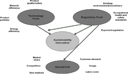
86 |
M. Wagner |
Fig. 5.2 Influencing factors of sustainability innovations and their interaction (Extended from Rennings 2000)
including energy and surface area) per unit output, and a minimal release of toxic substances”. A similar but more concise definition is proposed by the Eco Innovation Observatory (EIO) (2010, p. 10: “Eco-innovation is any innovation that reduces the use of natural resources and decreases the release of harmful substances across the whole life-cycle”). This definition can by analogy also be extended to the social domain. As stated before, innovations can be further differentiated by their level and whether processes, products or services are concerned.
One important factor affecting sustainability innovation is technological determinants. For instance, such a technological trend is represented by continuously increasing energy efficiency. Market influences, especially demand side and consumer preferences, are a further element. In addition to this, a major influence of regulation can be identified which may trigger and accelerate innovations or push the diffusion of already implemented innovation (Fig. 5.2). Financial incentives such as governmental subsidies and tax relief also support sustainable innovation. Broadly speaking, product innovations are mostly driven by market demand in terms of both the development of new products and the improvement of existing products. Conversely, regulatory requirements are more important for process innovations because they often initiate the development of these (Rennings 2000). Figure 5.2 summarises the three different determinants and shows their interaction and especially the moderating effect that regulation often has on market pull and technology push.
The considerations raised so far have led to the following research questions that will be addressed in the analysis:
1.What is the role of institutional/regulatory factors in the interaction of business strategies and sustainability innovation?
5 The Role and Effectiveness of Environmental and Social Regulations. . . |
87 |
2.Do lead markets exist where firms preferably introduce innovations that contribute much to sustainability, and what role does regulation have in the diffusion processes related to this?
3.Under which conditions do firms benefit most from innovation activities induced by regulation with regard to economic performance and competitive advantage?
4.What are the policy implications of the answers to the previous questions, especially with regard to the role of regulation in fostering diffusion versus innovation?
5.3Data and Methods
The data that the results are based on was derived from an analysis of manufacturing firms in a multi-method design. Initially, exploratory case interviews were carried out to gain a better understanding of qualitative links, and secondary data sources such as websites, corporate reports or newspaper articles were also used. Interviews were either in person or via telephone, lasted 0.5–2 h and were taped and subsequently transcribed in most cases.
Subsequently, German survey data was analysed to corroborate these links at a more representative level. The focus of research and methodology is detailed twostage case studies consisting of qualitative as well as quantitative data and statistical analysis. In the first qualitative stage, relevant resource domains and influencing factors are identified and classified. The second quantitative stage more formally tests the role of drivers in regulation-based sustainability innovations by means of multinomial logit regression based on survey data. Around 580 German manufacturing firms were invited by electronic mail to participate by completing questionnaire accessible on the internet. Of these firms, 169 responded, resulting in a response rate of 30 %. To assess the representativeness and response bias, the procedures suggested by Armstrong and Overton (1977) were adopted. Comparing the earliest and latest 10 % of respondents, no significant differences in the mean values of the responses for all variables were found other than late-responding firms being significantly smaller (see Wagner (2011) for more details on the survey content).
As a novelty, innovation offsets relating to product and process offsets can be separated in the data presented here. This is important since innovation offsets through products such as higher quality, safer products or higher scrap value versus process offsets such as material savings or lower handling costs may well be of differing importance. Parallel to this, existing strategy approaches are refined and combined by linking Porter’s traditional market-related management model with resource-based theory in terms of a structural model to arrive at a more integrative way of dealing with management issues affected by regulations. The section at the end evaluates the empirical evidence particularly with regard to the question of if, and to what extent, innovation offsets require investments in specific resource domains and whether these investments are triggered by regulations.
88 |
M. Wagner |
5.4Results
5.4.1Case-Based Analysis
From the case analysis and comparison, a number of salient results emerged. For example, with regard to the role of institutional/regulatory factors, it emerged that guidelines for energy efficiency in construction sector may on the one hand lead to innovation in the construction sector such as novel building materials or techniques such as the introduction exterior insulation and finish systems. On the contrary, regulations aimed at fostering energy efficiency were also found to imply safety and liability issues that made them obstacles for sustainability innovation. This became very clear in the construction industry with regard to architects who are hesitant to make use of or apply sustainability innovations due to additional legislation especially aimed at addressing liability and warranty concerns.
On the other hand, it has been confirmed in many cases that environmental or social aspects are perceived conventional goals or additional constraints of normal innovation processes. In terms of the dominant design, the analysis generally finds support for the stylised facts of innovation economics. For example, in the automotive industry, after dominant design, incumbents perform better with regard to innovation, whereas entrants are more successful before establishment of the dominant design. Specifically, entrants pursue radical product innovation, and incumbents’ incremental product innovation before the dominant design emerges in the automotive industry, whereas after its emergence, entrants appear to shift to a mix of radical and incremental process innovation and incumbents to mainly incremental process innovation. With regard to the types of innovation offsets that regulation can bring about, the following were identified:
•First-mover advantage (in new markets), export opportunities
•Certainty of future demand and a reliable investment climate
•Regulations as weak signals for long-term R&D strategies where small R&D efforts can be leveraged into high R&D returns in novel areas
•Unique selling propositions, premium prices
•Positive spillover effects from regulations in worldwide activities
•Increased awareness, reputation of the firm, and heightened ability for firms to push for standardisation with demanding standard levels
•Stronger interaction and cooperation of customers and suppliers
•Generation of intellectual property (e.g. patents)
As concerns lead markets, the qualitative evidence suggests that regulation helps to diffuse green or social features from high-end to low-price product categories and in doing so helps to create lead markets. One prominent example in Germany that emerged from the analysis is the feed-in law for electricity, the so-called Erneuerbare-Energien-Gesetz (EEG). Other legal means to achieve the same result that emerge from the case studies are taxes, subsidies and trading systems. The specific success of the EEG appears to be due to the fact that it was a rare
5 The Role and Effectiveness of Environmental and Social Regulations. . . |
89 |
parliamentary initiative. Overall, the EEG significantly fostered the diffusion of renewable energy installations in Germany, but mainly had indirect innovation effects in that it accelerated moving along experience and learning curves, subsequently leading to price declines and increased competitiveness (see Costantini and Crespi (2010) on similar issues). Generally, it also seems that the stronger effect of regulation on diffusion that was identified here is also due to the phenomenon that research and development are often pursued before a regulation is enforced. This is part of a learning process that a firm undergoes in terms of positioning itself towards a regulation by means of research itself (a special case of learning-by-doing). This suggests a co-evolution of regulation and innovation activity at the fuzzy front-end of the regulation-innovation nexus. Often it does not seem to be clear when firms actually started innovating. A co-evolution is also likely because firms are more inclined to push for regulation once they have a lead in innovation. It could be interesting to address this question further by measuring sustainable innovation through patent classes, even though this is in some respects an issue and potentially even more so with the trend towards integrated technology solutions.
With regard to the conditions under which firms profit most from regulationdriven innovation, two main functions can be distinguished. First, there is the accelerator function which is embodied in forced fast switches (innovate or die), acceleration of ongoing R&D and the commercialisation of existing inventions. This function requires a safe investment climate and means of compensation for research and investment costs. Regulation in this increases awareness and as a result shifts the focus of innovation activities to sustainability innovations. Second, indirect effects exist which relate especially to interdependencies of customer and supplier markets and to planning security for production facilities. Third, different and differential effects from regulation emerge with the most frequently cited regulations being automotive emissions regulations and the RoSH and WEEE directives (see Mazzanti and Zoboli (2006) and Mazzanti et al. (2008) on this). On the one hand, firms gain experience in processing toxic materials and emissions and develop capabilities for designing and implementing better secondary treatment processes which reduce the cost of compliance for end-of-pipe pollution control. On the other hand, firms pursue innovation activities that improve products and processes and in doing so create innovation offsets that can exceed the initial cost of compliance with regulation.
5.4.2Survey Analysis
By extending and building on the case analysis, a structural model for determinants of regulation-driven innovation was developed and tested with firm-level data in the German manufacturing sector in the specific context of environmental and sustainability-related innovation. The results are summarised in Table 5.1.
The estimation results presented here are based on a multinomial logit model used in order to identify the main determinants governing whether sustainable
Table 5.1 Results of the model (T: technology, R: regulation driver, market demand)
|
|
T |
R |
T |
|
R |
|
T |
|
R |
|
T |
|
R |
|
1 |
Size |
0.03 |
0.08 |
0.01 |
|
0.09 |
|
0.04 |
|
0.01 |
|
0.07 |
|
0.02 |
|
|
|
(0.06) |
(0.07) |
(0.08) |
|
(0.08) |
|
(0.08) |
|
(0.08) |
|
(0.08) |
|
(0.09) |
|
2 |
Integration |
0.63 |
0.76 |
0.73 |
|
0.77 |
|
0.98 |
|
0.82 |
|
1.04 |
|
0.87 |
|
|
|
(0.30) ** |
(0.29) *** |
(0.34) |
** |
(0.33) |
** |
(0.38) |
*** |
(0.36) |
** |
(0.39) |
*** |
(0.36) |
** |
3 |
Business conditions |
0.01 |
0.27 |
0.16 |
|
0.01 |
|
0.43 |
|
0.26 |
|
0.60 |
|
0.42 |
|
|
|
(0.33) |
(0.31) |
(0.37) |
|
(0.35) |
|
(0.40) |
|
(0.38) |
|
(0.41) |
|
(0.40) |
|
4 |
EMS index |
0.07 |
0.06 |
0.07 |
|
0.15 |
|
0.21 |
|
0.22 |
|
0.21 |
|
0.21 |
|
|
|
(0.08) |
(0.08) |
(0.12) |
|
(0.10) |
|
(0.13) |
|
(0.12) |
* |
(0.13) |
|
(0.12) |
* |
5 |
QMS |
0.33 |
0.27 |
0.08 |
|
0.211 |
|
0.37 |
|
0.34 |
|
0.38 |
|
0.18 |
|
|
|
(0.62) |
(0.67) |
(0.74) |
|
(0.78) |
|
(0.82) |
|
(0.85) |
|
(0.85) |
|
(0.88) |
|
6 |
Concerned stakeholders |
|
|
0.05 |
|
0.55 |
|
0.21 |
|
0.60 |
|
0.27 |
|
0.68 |
|
|
|
|
|
(0.62) |
|
(0.60) |
|
(0.66) |
|
(0.65) |
|
(0.70) |
|
(0.67) |
|
7 |
Partly concerned stakeholders |
|
|
0.16 |
|
0.14 |
|
0.17 |
|
0.17 |
|
0.16 |
|
0.19 |
|
|
|
|
|
(0.53) |
|
(0.54) |
|
(0.55) |
|
(0.57) |
|
(0.56) |
|
(0.57) |
|
8 |
Unconcerned stakeholders |
|
|
0.49 |
|
1.72 |
|
0.69 |
|
1.66 |
|
0.70 |
|
1.59 |
|
|
|
|
|
(0.57) |
|
(0.60) |
*** |
(0.60) |
|
(0.63) |
*** |
(0.61) |
|
(0.64) |
** |
9 |
Independent firm |
|
|
0.31 |
|
0.61 |
|
0.43 |
|
0.76 |
|
0.62 |
|
0.98 |
|
|
|
|
|
(0.53) |
|
(0.51) |
|
(0.57) |
|
(0.54) |
|
(0.59) |
|
(0.56) |
* |
10 |
Share of green innovation patented |
|
|
0.02 |
|
0.00 |
|
0.02 |
|
0.01 |
|
0.02 |
|
0.01 |
|
|
|
|
|
(0.01) |
*** |
(0.01) |
|
(0.01) |
*** |
(0.01) |
|
(0.01) |
*** |
(0.01) |
|
11 |
Green processes implemented |
|
|
1.21 |
|
0.48 |
|
1.17 |
|
0.64 |
|
1.10 |
|
0.62 |
|
|
|
|
|
(0.64) |
** |
(0.59) |
|
(0.67) |
* |
(0.63) |
|
(0.68) |
|
(0.64) |
|
12 |
Green products developed |
|
|
1.28 |
|
1.42 |
|
1.74 |
|
1.81 |
|
1.95 |
|
1.96 |
|
|
|
|
|
(0.58) |
** |
(0.56) |
*** |
(0.63) |
*** |
(0.63) |
*** |
(0.67) |
*** |
(0.64) |
*** |
13 |
Breadth |
|
|
|
|
|
|
1.13 |
|
0.27 |
|
1.32 |
|
0.32 |
|
|
|
|
|
|
|
|
|
(0.66) |
* |
(0.61) |
|
(0.72) |
* |
(0.63) |
|
14 |
Quality |
|
|
|
|
|
|
1.22 |
|
0.89 |
|
1.13 |
|
1.00 |
|
|
|
|
|
|
|
|
|
(0.76) |
|
(0.76) |
|
(0.77) |
|
(0.77) |
|
15 |
Focus |
|
|
|
|
|
|
2.99 |
|
2.57 |
|
2.93 |
|
2.67 |
|
|
|
|
|
|
|
|
|
(0.93) |
*** |
(0.89) |
*** |
(0.94) |
*** |
(0.90) |
*** |
16 |
R&D intensity |
|
|
|
|
|
|
|
|
|
|
0.21 |
|
0.20 |
|
|
|
|
|
|
|
|
|
|
|
|
|
(0.14) |
|
(0.15) |
|
Notes: *p < 0.1; **p < 0.05; ***p < 0.01, T technology, R regulation; industry dummies at 2-digit SIC level are included in all models; when R&D intensity was unavailable, a missing R&D dummy was used to enable estimation in accordance with the method proposed by Hall and Ham Ziedonis (2001)
90
Wagner .M
5 The Role and Effectiveness of Environmental and Social Regulations. . . |
91 |
innovation is technology or regulation driven (rather than being market driven). The independent variables for all models were based on prior empirical work in industrial economics (Schmalensee 1989; Wagner 1992, 1995), innovation economics (Ziegler and Rennings 2004; Tidd et al. 2005) and environmental management research (Wagner and Schaltegger 2004; Wagner 2008). They include a significant number of explanatory factors such as firm size, existence of a quality management system (a dummy variable taking the value 1 if the firm has ISO 9001) and firm legal structure. Next to these additional environmental management variables, stakeholder variables and prior innovation variables are included. As can be seen in Table 5.1, being more regulation driven, innovation is significantly positively associated (i.e. more likely) with a firm being independent, prior green product development; a firm pursuing a focussed strategy in the sense of Porter (1985); or a firm with high levels of environmental management system (EMS) implementation. Furthermore, it is more likely that innovation is induced by the market rather than by regulation being induced by regulation, if a firm experiences stronger pressure from stakeholders that are not concerned with sustainability issues and a firm has higher levels of integration of sustainability with strategic aspects of the business. These results suggest that stronger integration leads to stronger market orientation (i.e. innovation is more driven by market demand than by regulatory requirements) and the same applies for stakeholders that are not particularly concerned about sustainability (i.e. social benefits) but purely about their private benefits (which can be adequately captured in markets). Similarly, if firms have firm internal resources and capabilities for sustainable innovation (such as high levels of EMS implementation that enable early detection of regulatory requirements or past eco-innovation experience), then their sustainable innovation activities are more strongly receptive to regulation. Interestingly, this also applies to firms pursuing focussed differentiation or focussed cost-leadership strategies which could be due to better knowledge of the more narrow market segments that such firms cater for. Analyses could be carried out with regard to specific innovation offsets on a subset of the firms responding to the survey. This is the case for 55 survey responses. Of these, the majority confirms innovation offsets (Table 5.2).
Double as many instances of process innovation were observed compared with product innovation so that regulations appear to largely drive process innovation. With regard to the type of offsets and the distinction between product and process offsets, in particular, as can be seen in Fig. 5.3, the analysis generally confirmed that regulation pushes innovation with the most frequent offsets observed being increased product performance and material savings (in Fig. 5.3 more than one offset could be named).
Occurrence and the level of innovation depend on the specific regulation with the most significant effects in Europe emerging from REACH and the EU Noise Directive – for the latter, however, mainly for less radical innovation. Radicality was defined here in terms of small to large modifications to new-to-the-world products or processes (Wagner 2011) with the share of these categories in the responses being provided by Fig. 5.4.
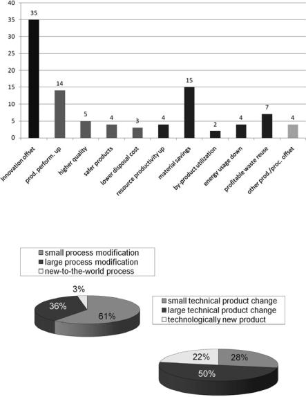
92 |
|
M. Wagner |
Table 5.2 Share of stringent regulation triggering innovation |
|
|
|
|
|
Regulation type/innovation occurrence |
Innovation triggered |
Innovation not triggered |
|
|
|
Regulation stringent |
35 |
13 |
Regulation not stringent |
2 |
5 |
Fig. 5.3 Distribution of innovation offsets across different categories
Fig. 5.4 Distribution of innovation levels for product and process innovation
5 The Role and Effectiveness of Environmental and Social Regulations. . . |
93 |
Generally, no significant association is found between firms pursuing green product or process innovation and firms with green patents or patents in general (Wagner 2007). There is also no significant association with the amount of patents. Furthermore, no significant association between the level of green product or process innovation and the existence of green patents or patents in general or the amount of patents is found.
5.5Conclusions
Overall, the research study reported here suggests that both institutional and regulatory factors play a role in sustainability innovation and also shape their interaction with business strategies. As the analysis shows, ambitious sustainability strategies of businesses often build on sustainability innovation as a core element. Institutional factors such as a firm being independent make it more likely that they will perceive their innovation activities as being mainly regulation driven. The situation can thus be understood as a co-evolving system of regulatory demands and institutional factors needed to meet these demands in which both aspects need to be balanced. Related to this, the analysis also reveals complementarities (or at least co-dynamics) both within the firm and in its socio-economic context. Whereas the latter mainly concerns the interaction of market demand and regulation (especially in the context of innovation diffusion), the former is broadly related to the complementarity of bottom-up and strategic routines.
The analysis also shows that lead markets exist where firms introduce sustainability innovations at greater speed. Regulation often appears to create these lead markets (e.g. in Germany, the Erneuerbare-Energien-Gesetz (EEG) which fosters the input of decentrally generated renewable electricity to the power grid). Here, regulation seems to have an important but so far largely neglected role in the diffusion of sustainability processes which goes beyond triggering or fostering invention and is often implemented by means of lead markets.
With regard to the conditions under which firms benefit most from innovation activities induced by regulation as far as economic performance and competitive advantage is concerned, the analysis shows that conflicts between economic and ecological/social objectives of firms can exist, but it is not possible to identify whether innovation behaviour differs in technologies according to the degree to which economic, ecological and social aspects are treated in an integrated manner. Regulations can also support investments in existing technologies rather than the development of novel sustainable innovations. These investments also affect the way regulatory uncertainty or stringency slows down or speeds up sustainability innovation as a whole. By building up internal capabilities and competencies in time (making use of bottom-up activities and strategic routines simultaneously), corporations can profit from accelerating functions of anticipated regulatory strengthening by bringing forward already invented innovations, for example.
94 |
M. Wagner |
Both for-profit and for-benefit firms also have in principle advantages from regulations such as subsidies, feed-in tariffs and other market-based instruments.
With regard to the policy implications of the findings, a framework function can first be identified in that a clear regulatory framework supports a long-term innovation strategy with significant R&D efforts. In this function, strict limits reduce uncertainty and increase a company’s awareness. Second, an accelerator function can be identified that relates especially to the role of regulation in pushing diffusion of innovation versus invention and to learning curve effects where simultaneous use of voluntary standards helps to coordinate learning processes. Finally, the question of the regulatory optimum seems relevant given the insights in the construction industry. From this perspective, it is important to minimise the hindering effect of regulation and maximise their positive innovation effects which may additionally be achieved by a strong framework.
References
Armstrong, J. S., & Overton, T. S. (1977). Estimating non-response bias in mail surveys. Journal of Marketing Research, 14, 396–402.
Costantini, V., & Crespi, F. (2008). Environmental regulation and the export dynamics of energy technologies. Ecological Economics, 66, 447–460.
Costantini, V., & Crespi, F. (2010). Public policies for a sustainable energy sector: Regulation, diversity and fostering of innovation. Journal of Evolutionary Economics. doi:10.1007/ s00191-010-0211-3.
Costantini, V., & Mazzanti, M. (2012). On the green and innovative side of trade competitiveness? The impact of environmental policies and innovation on EU exports. Research Policy, 41, 132–153.
EIO Eco Innovation Observatory. (2010). Methodological report for the European. Brussels: Europe Innova.
Hall, B. H., & Ham Ziedonis, R. (2001). The patent paradox revisited: An empirical study of patenting in the U.S. semiconductor industry, 1979–1995. The RAND Journal of Economics, 32, 101–128.
Hart, S. (1995). A natural-resource-based view of the firm. Academy of Management Review, 20, 986–1014.
Lanjouw, J., & Mody, A. (1996). Innovation and the international diffusion of environmentally responsible technologies. Research Policy, 25, 549–571.
Mazzanti, M., & Zoboli, R. (2006). Economic instruments and induced innovation: The EU policies on end of life vehicles. Ecological Economics, 58, 318–338.
Mazzanti, M., Montini, A., & Zoboli, R. (2008). Municipal waste generation, socio-economic drivers and waste management instruments. Journal of Environment and Development, 17, 51–69.
Porter, M. (1985). Competitive advantage. New York: The Free Press.
Porter, M., & van der Linde, C. (1995). Toward a new conception of the environmentcompetitiveness relationship. Journal of Economic Perspectives, 9, 97–118.
Reid, A., & Miedzinski, M. (2008). Sectoral innovation watch in Europe – Eco-innovation. Brussels: Europe Innova.
Rennings, K. (2000). Redefining innovation — Eco-innovation research and the contribution from ecological economics. Ecological Economics, 32, 319–332.
5 The Role and Effectiveness of Environmental and Social Regulations. . . |
95 |
Schmalensee, R. (1989). Inter-industry studies of structure and performance. In R. Schmalensee & R. D. Willig (Eds.), Handbook of industrial organization (pp. 951–1009). Amsterdam: North Holland.
Tidd, J., Bessant, J., & Pavitt, K. (2005). Managing innovation. London: Wiley.
Wagner, J. (1992). Firm size, firm growth, and persistence of chance: Testing Gibrat’s law with establishment data from Lower Saxony, 1978–1989. Small Business Economics, 4, 125–131.
Wagner, J. (1995). Firm size and job creation in Germany. Small Business Economics, 7, 469–474. Wagner, M. (2007). On the relationship between environmental management, environmental innovation and patenting: Evidence from German manufacturing firms. Research Policy, 36,
1587–1602.
Wagner, M. (2008). The influence of environmental management systems and tools on innovation: Evidence from Europe. Ecological Economics, 66, 392–402.
Wagner, M. (2011). Sustainability-related innovation and competitiveness-enhancing regulation: A qualitative and quantitative analysis in the context of open innovation. International Journal of Innovation and Sustainable Development, 5, 371–388.
Wagner, M., & Schaltegger, S. (2004). The effect of corporate environmental strategy choice and environmental performance on competitiveness. European Management Journal, 22, 557–572.
Ziegler, A., & Rennings, K. (2004). Determinants of environmental innovations in Germany: Do organizational measures matter? (ZEW Working Paper). Mannheim: ZEW.
Part II
Environmental Innovation and
Competitiveness: Linking Micro, Meso and
Macro Analysis in the Dynamics

Chapter 6
Implications of Policy Uncertainty for Innovation in Environmental Technologies: The Case of Public R&D Budgets
Margarita Kalamova, Nick Johnstone, and Ivan Hasˇcˇicˇ
Abstract The role that environmental policy uncertainty can play on innovation in environmental technologies has not been extensively assessed empirically. In this chapter, we seek to assess the impact of environmental policy uncertainty on innovation, using patent data as a proxy for innovation and volatility in public expenditures on ‘environmental’ R&D as a measure of policy uncertainty. Drawing upon a panel data set of 23 OECD countries over the period 1986–2007, support is found for the negative effect of public R&D volatility on innovation. In the base model, a 10% increase in policy uncertainty is seen to cause a 1.2–2.8% decrease in environmental patent activity, whereas a 10% increase in government support for R&D will increase innovation by 2.6–3.9%.
Keywords Policy uncertainty • Innovation • Public R&D • Patents • OECD
The views expressed here are the authors’ own and do not necessarily reflect those of the OECD or its members.
M. Kalamova • I. Hasˇcˇicˇ
Organisation for Economic Co-operation and Development, OECD Environment Directorate, 2 rue Andre Pascal, 75775 Paris Cedex 16, France
e-mail: Margarita.Kalamova@oecd.org; Ivan.Hascic@oecd.org
N. Johnstone (*)
Organisation for Economic Co-operation and Development, OECD Environment Directorate, 2 rue Andre Pascal, 75775 Paris Cedex 16, France
Empirical Policy Analysis Unit, OECD Environment Directorate, 2 rue Andre´-Pascal, 75775 Paris Cedex 16, France
e-mail: Nick.Johnstone@oecd.org
V. Costantini and M. Mazzanti (eds.), The Dynamics of Environmental |
99 |
and Economic Systems: Innovation, Environmental Policy and Competitiveness,
DOI 10.1007/978-94-007-5089-0_6, # Springer Science+Business Media Dordrecht 2013
100 |
M. Kalamova et al. |
6.1Introduction
The importance of uncertainty and irreversibility on investment has been well researched in the theoretical literature. However, for some time, these factors seemed to be missing from most empirical research on investment and have created a ‘somewhat disturbing gap between theory and empiricism’ as noted by Pindyck (1991a). While this gap has been filled, some areas remain for which empirical evidence is limited. In particular, the role that environmental policy uncertainty can play on innovation in environmental technologies has not been extensively assessed empirically.
In this chapter, we seek to assess the impact of environmental policy uncertainty on innovation, using patent data as a proxy for innovation and volatility in public expenditures on ‘environmental’ R&D as a measure of policy uncertainty. Indeed, the policy framework in pollution and resource-intensive sectors can be one of the most important factors in the investment decision. For instance, investors in waste-intensive sectors in Europe need to anticipate forthcoming directives which will have an effect on their capital investments. In the context of climate change, the issue may be even more important since government commitments are the outcome of both domestic and international negotiations. In such cases, there can be strong incentives to wait until ‘the policy dust settles’ before adopting a specific investment strategy.
The potential effect of environmental policy uncertainty on incentives to invest in environmental technology arises from the real options literature (see Dixit and Pindyck (1994) for the classic treatment; Pindyck (2007) discusses the specific case of environmental investments). The value of an investment project depends on future output prices, input costs, interest rates, etc. The opportunity cost of the option to invest is a significant component of the firm’s investment decision. The option value increases with the sunk cost of the investment and with the degree of uncertainty over the future price. As Dixit and Pindyck (1994) show in this case, the option to invest will be exercised when output prices exceed the cost of input by an amount equal to the value of keeping the investment option alive. Hence, fluctuations in the value of a project can be traced back to uncertainty in these more basic variables.
The findings of the option-value literature are particularly relevant in the context of investment in innovative activities, such as investment in R&D, because such investments are by nature almost irreversible. Since the costs of these investments cannot usually be recovered if market conditions change, market uncertainty can serve as a significant brake on investment in innovative activities. For instance, in a panel data study of nine OECD countries covering the period 1981–1992, Goel and Ram (2001) find a much sharper adverse effect of uncertainty on R&D investments than on non-R&D (and aggregate) investments. Almost all R&D expenditure on personnel, equipment and materials is irreversible since it is particularly firmspecific or industry-specific, or has the lemons problem as noted by Pindyck (1991b). Thus, irreversibility of investment accentuates the adverse effect of uncertainty (Pindyck 1991b; Dixit and Pindyck 1994).
Importantly, market uncertainty can be compounded by policy uncertainty. For instance, Dixit and Pindyck (1994) show that a case for policy intervention will

6 Implications of Policy Uncertainty for Innovation in Environmental Technologies. . . |
101 |
arise only if firms face a different value of waiting than society as a whole (i.e. if some market failure is associated with the decision process). They study the effect of uncertainty concerning future policy itself and discuss the example of an investment tax credit. They assume that firms will attach more value to waiting because there is a probability that the cost of investment to the firm will fall and find that this policy uncertainty can have a powerful deterrent effect on immediate investment. They conclude that if governments wish to stimulate investment, perhaps the worst thing they can do is to spend a long time discussing the right way to do so. Rodrik (1991), among others, shows that if each year there is some probability that the policy will be reversed, the resulting uncertainty can eliminate any stimulative effect that the policy would otherwise have had on investment. The public economics literature generally confirms the conventional wisdom that tax policy uncertainties can adversely affect firms’ incentives to invest.1
Environmental policy uncertainty has become a significant concern of late. By imposing a price (either explicitly or implicitly) on the costs of pollution emissions, environmental policy is likely to induce innovation as firms seek to meet the policy objectives at least cost. However, if there is uncertainty concerning the stringency, nature and timing of the policy introduced, this can encourage potential innovators to wait before undertaking the necessary investments. It is important to note that environmental policy uncertainty will arise even in an optimal policy setting.
On the one hand, this may be due to uncertainty concerning environmental damages. With unknown damages and increasing information through time, policy conditions may change as the magnitude of the benefits of policy interventions become better known. For instance, there is a large and growing body of literature on the implications of uncertainty regarding climate change damages on the optimal degree of stringency of environmental policy (Baker and Adu-Bonnah 2008). On the other hand, uncertainty with respect to technological conditions may lead to changing environmental policy conditions. Factor substitution possibilities may not be known with any degree of certainty. For instance, in the US Acid Rain Program, the difference between ex ante and ex post estimates of abatement costs has been considerable (Burtraw and Palmer 2004). As such, the optimal level of policy stringency may also change as policymakers acquire information on market responses.
Empirical evidence is mixed concerning the impact of damage and technological uncertainty on the optimal level of investment in R&D on environmental technologies (Baker and Shittu (2006) review much of the recent literature on these two sources of uncertainty in the context of climate policy models). However, the effect of actual policy uncertainty on innovation in environmental technologies has not been examined empirically, although Yang et al. (2008) assess the effects of climate policy uncertainty or fuel choice. In particular, if the future trajectory of this cost is uncertain, option-value theory indicates that individual firms may choose to wait before undertaking investments which seek to identify the means of reducing this cost (i.e. before investing in environmental R&D). Since expectations concerning environmental policy are one of the key determinants of
1 Studies exploring this effect include Rodrik (1991) and Aizenman and Marion (1993), among others.
102 |
M. Kalamova et al. |
perceived uncertainty over the firm’s planning horizon, policy predictability can play an important role in inducing environmental innovation. In this chapter, we seek to examine formally the proposition that policy uncertainty has slowed investment in environmental innovation. Specifically, drawing upon a database of patent applications from a cross section of 23 OECD countries over the time period 1986–2007, evidence is provided for the negative effect of policy uncertainty of the domestic environmental policy regime on the rate of innovation for environmental technologies. Contrary to previous studies, this chapter makes a novel attempt to measure policy uncertainty by using the coefficient of variation of public R&D expenditures as a proxy for uncertainty.
6.2Policy Uncertainty and Investment Irreversibility
As noted above, compliance with environmental regulation is often a moving target as environmental regulations are likely to evolve over time. Yet, an investment, once made, has aspects of irreversibility and reversing a regrettable choice is costly (Purvis et al. 1995). Hence, uncertainty over the policy regime can affect incentives to develop and adopt environmental technologies. This policy uncertainty can take different forms:
•Uncertainty concerning the stringency of the policy and thus the ‘price’ associated with polluting
•Uncertainty concerning the timing of the introduction of the policy and thus the point at which a ‘cost’ is incurred
•Uncertainty concerning the nature of the instrument to be used and thus the means by which the cost is incurred
•Uncertainty concerning the ‘durability’ of the policy and thus the horizon over which the price can be assumed to be in place
There are a small number of studies that address one or more of these aspects of environmental policy uncertainty, indicating that both the rate and direction of innovation can be significantly affected by policy uncertainty.
For instance, there is significant anecdotal evidence in the area of renewable power development to support the hypothesis that uncertainty concerning the time horizon over which investors foresee a given policy to remain in place has played at least as important a role as policy stringency (So¨derholm et al. 2007; Wiser and Pickle 1998; Barradale 2008). In particular, Barradale (2008) argues that in the case of the United States, uncertainty concerning annual renewal of the federal production tax credit (PTC) discouraged investment in renewable energy. This finding is supported by anecdotal evidence presented in Wiser and Pickle (1998) concerning both wind and solar power. In a comparison of wind power development in Denmark, Germany and Sweden, So¨derholm et al. (2007) argue that the relatively slow pace of development in Sweden is due to instability in the policy framework more than the actual level of support, with a number of different subsidy programmes implemented successively for short periods of time. Interestingly,

6 Implications of Policy Uncertainty for Innovation in Environmental Technologies. . . |
103 |
Barradale (2008) provides evidence that perceived uncertainty is correlated with instrument choice. Investors in the sector believed that renewable energy portfolio standards were more likely to stay in effect long enough to influence long-term investment decisions than depreciation rules, tax credits, feed-in tariffs or production subsidies (which all have direct implications for public budgets).
Isik (2004) analyses the extent to which uncertainty over cost-share subsidy policies aimed at achieving pollution reductions by accelerating the adoption of different farming systems and new technologies in agriculture would impact farmers’ adoption decisions using an option-value model. The author showed that an increase in the probability of an expected public policy leads farmers to delay the adoption of new technologies in order to learn more about market conditions and the value of these technologies. Furthermore, cost-share subsidy policies are found to be more effective when they are immediately offered to farmers and a guarantee provided that they will be removed soon.
Uncertainty concerning the nature of the instrument to be implemented can also have an effect on the rate and nature of innovation. Even if a government is committed to a given environmental objective and provides a credible time frame for its achievement, investors are likely to delay investment until the precise form of the policy instrument is proposed. This is particularly important if the policy options that the government has at its disposal include technology-based standards. In such circumstances, the investor runs the risk of ending up with significant stranded assets if the specific abatement technology is not consistent with permit requirements. The risk is much less if more flexible instruments are introduced. However, even in the case of performance standards, the risk can be considerable if the abatement option adopted does not allow for ex post adjustment of performance levels.
Regulatory uncertainty can also affect the direction of innovation. When choosing between alternative abatement options, the firm must assess the cost of initial capital investment, operating costs and the costs of adjusting production technologies in the face of changing policy conditions. It is important to note that the cost of adjusting production technologies reflects any additional expenditures incurred, minus any salvage value obtained from the resale of capital equipment which is no longer of value to the firm.2 Interestingly, despite regulatory uncertainty, there may be an incentive to invest in end-of-pipe (EOP) abatement rather than more integrated changes in production processes (CPP), even if the latter is a more cost-effective means of mitigating pollution. In the former case (EOP), the abatement decision can be ‘hived off’ from more general production decisions, reducing the probability of being left with stranded assets if there is a change in policy conditions.
The case of coal-fired electricity generation is particularly interesting in this respect. In the face of existing or potential constraints on CO2 emissions, investors in coal-fired electricity generation face a choice between investment in advanced
2 Note that the resale value may be zero if the capital is specific, and the regulatory change impacts on all potential adopters.
104 |
M. Kalamova et al. |
pulverised coal (APC) or integrated gasification and combined cycle plants (IGCC). The capital costs for the former are somewhat lower than for the latter. However, the costs of retrofitting for carbon capture and storage (CCS) are much higher for APC than for IGCC (Bohm et al. 2007). In the presence of regulatory uncertainty over future carbon prices or CCS requirements, there is a value attached to investing in the more ‘flexible’ capital equipment (IGCC). However, uncertainty will slow the delay of the retirement of existing (and more polluting) facilities. Indeed, in a numerical simulation model, Reinelt and Keith (2007) find that under plausible assumptions emissions may be higher when there is regulatory uncertainty than when there is certainty that no regulation will be introduced. The social costs generated can be considerable.
There are a small number of studies that have assessed the role of cost uncertainty arising from either changes in the regulatory regime or volatility inherent to the regulation itself (i.e. permit price volatility or changes in tax levels). For instance, Fuss et al. (2008) also examine the CCS investment decision but focus on the difference between market-driven price uncertainty and policy-driven price uncertainty. The latter is measured as a discrete break in the CO2 price trajectory. They find that market-driven price uncertainty may result in earlier investment in CCS than under conditions of no price uncertainty. However, policy-driven price uncertainty will always delay the CCS investment decision.
Xepapadeas (2001) defines uncertainty as stochastic movements of tradable emissions prices or unpredictable (from the firms’ point of view) policy changes. Moreover, the author accounts for the irreversibility of abatement investment expenses. His analysis yields implications for the regulator concerning the optimal policy design: a regulator can design a policy scheme consisting of two instruments – an emissions tax or tradable permit system and a subsidy on abatement investment. The policy scheme takes uncertainty into account through its dependence on the parameters of the price process and will induce individual firms to undertake the same output and abatement investment under uncertainty that a regulator would have undertaken. Farzin and Kort (2000) theoretically analyse the effects of uncertainty over the size of a tax increase at a certain future date and uncertainty over the timing of a known tax increase. Their results suggest that though both types of uncertainties affect the optimal abatement investment path, the effect of the former may be more pronounced, especially when investment is irreversible. Interestingly, they show that a credible threat of accelerating the tax increase can further boost the firm’s abatement investment.
In one of the few formal empirical studies, Lo¨fgren et al. (2008) assess Swedish firms’ investments in pollution abatement technology related to SO2 emissions. In their model, the price of the polluting fuel is the major source of uncertainty facing the firm, drawing upon a panel of firms from the Swedish pulp and paper industry and the energy and heating sector, and their sulphur dioxide emissions over the period 2000–2003. The results indicate that in the presence of uncertainty over the price of the polluting fuel, the hurdle rates – i.e. the multiplier of the price of the polluting fuel relative to a condition of perfect information necessary to trigger investment in the less pollution technology – are between 2.7 and 3.1 for the pulp
6 Implications of Policy Uncertainty for Innovation in Environmental Technologies. . . |
105 |
and paper sector and 3.4 and 3.6 in the energy and heating industry. Interestingly, they note that there are differences between firms that invest in EOP vs. CPP technologies, but no firm conclusions are drawn regarding the role of uncertainty in guiding the decision.
In a study on the US pulp and paper sector, Maynard and Shortle (2001) assessed the effect of protracted uncertainty concerning the development of the US EPA’s Cluster Rule (which targeted dioxins) on adoption of less polluting technologies. They examined three abatement options: extended delignification (ED), oxygen delignification (OD) and more advanced elemental chlorine-free bleaching (ECF). The different options have interesting characteristics. While ED and OD are more integrated in the production process than ECF, which can be considered a form of end-of-pipe technology, the cost of implementing ECF is less if the plant already has invested in ED or OD. Using a double-hurdle model, they find that the uncertainty surrounding the policy encouraged investors to ‘wait and see’ before undertaking the investments in both extended or oxygen delignification or elemental chlorine-free bleaching. Prior investment in ED or ED affected the decision to invest in ECF.
Theoretical arguments and empirical evidence indicate that the effects of frequent and unpredictable policy changes on long-term investments can, therefore, be considerable.
6.3Hypothesis
In the environmental context, unlike many other areas, the viability of a specific investment is dependent upon a specific policy regime remaining in place. This is a major risk that inventors will need to evaluate before deciding on the investment project. Companies must absorb significant risk during the research and development phase of a product if there is some uncertainty that a particular policy will apply to their project when it becomes commercially viable. Even where policies survive, attempts at legislative intervention, agency and/or court rulings can significantly alter a policy’s applicability and implementation. Since unpredictability of these policies provides some uncertainty to the profitability of innovation efforts, companies will be reluctant to innovate. The empirical hypothesis can therefore be stated as follows: Uncertainty over environmental policy will have a negative impact on a firm’s decision to innovate in environmental technologies.
Our measure of innovation is counts of patent applications for environmental technologies, discussed in further detail below. As a measure of policy uncertainty, we use volatility in public expenditures on environmental R&D. This includes both direct government expenditures for R&D undertaken in government and publicly funded university laboratories as well as the provision of financial support (grants, tax credits, etc.) for R&D undertaken by the private sector and other organisations.
This measure should reflect at least two aspects of uncertainty. First, since some form of public fiscal support is usually necessary for privately undertaken R&D

106 |
M. Kalamova et al. |
projects in environmental technologies to be feasible at all, this measure will reflect variation in the cost of the investment. Second, since public R&D targeted at a specific field can be considered as a signal of related public policy objectives, volatility in such expenditures can be used as a measure of commitment.
6.4Data and Empirical Analysis
In this study, patent data are used to construct a proxy measure of environmental innovation. Patent data have been used as a measure of technological innovation because they focus on outputs of the inventive process (Griliches 1990; OECD 2009). This is in contrast to many other potential candidates (e.g. research and development expenditures, number of scientific personnel) which are at best imperfect indicators of the innovative performance of an economy since they focus on inputs. Moreover, patent data provide a wealth of information on the nature of the invention and the applicant; the data is readily available and discrete (and thus easily subject to statistical analysis). Significantly, there are very few examples of economically significant inventions which have not been patented (Dernis et al. 2001).
The data used to construct this indicator were taken from the OECD Patents Statistics database3 based on counts of patent applications in key areas of environmental technology – air pollution abatement, water pollution abatement, solid waste management, soil remediation and environmental monitoring technologies. (See Appendix for a list of IPC classes used to identify the relevant patented inventions.) The dependent variable represents the number of patent applications deposited at the European Patent Office, classified by inventor country4 and priority year.5 To test the empirical hypothesis, the following model is estimated:
ENVPATi;t ¼ f ðTOTAL PATENTSi;t; GBAORDENVi;t ; POLICY UNCERTAINTYi;tÞ þ ei;t
(6.1)
where i indexes country and t stands for year. The dependent variable is measured by the number of patent applications in environmental technology as described above.
It is important to control statistically for differences in the propensity to innovate and patent across countries. In order to capture the effect of such factors (which are not specific to environmental technologies), we include the variable TOTAL PATENTS reflecting the total number of patent applications deposited at the EPO
3http://stats.oecd.org/index.aspx?queryid¼29068
4‘Fractional’ counts are generated in cases when inventors from multiple countries are listed.
5‘Priority date’ indicates the earliest application date worldwide (within a given patent family).

6 Implications of Policy Uncertainty for Innovation in Environmental Technologies. . . |
107 |
filed across the whole spectrum of technological fields (not only environmental). This variable thus controls for differences in a country’s general research capacity as well as changes in general propensity to patent over time and across countries. Ideally, we would estimate the model using a two-stage procedure where total patenting activity is first estimated. This approach was followed (Johnstone et al. 2012) and results from the two-stage estimation were seen to be closely comparable with those from a reduced-form model. Since many observations would be lost with such an approach, in this case, we have decided to adopt this strategy.6 The sign on this variable is expected to be positive.
In previous work on the determinants of environmental innovation, relative policy stringency has been included as the principal environmental policy factor (Brunnermeier and Cohen 2003; Lanjouw and Mody 1996; Johnstone et al. 2010). The relative stringency of environmental policy is thought to induce innovation by changing relative factor prices or introducing production constraints (Hicks 1932). However, measurement of this effect is complicated because cross-country (or cross-sectoral) data on regulatory stringency are rarely available or are not commensurable. Moreover, public policies typically target specific environmental impacts (pollutants) using a specific policy instrument. This chapter deals with a broadly defined (environmental) technology and hence covers multiple impacts and potentially a wide spectrum of policy instruments and sectors. Moreover, it operates in a cross-country context. Previous studies have used data on pollution abatement and control expenditures of the private sector (PACE) as well as on perceived stringency (survey by the World Economic Forum) to measure the stringency of environmental policy regimes. However, the first variable consists of large numbers of missing observations, whereas the second one is available for a very short period of time only (2001–2007).
As noted, in this study, we use government budget appropriations and outlays for R&D (GBAORD). GBAORD data is disaggregated by socio-economic objective, including control and care of the environment7 (GBAORDENV). This is applied as a proxy of policy stringency. The data are taken from the OECD Research and Development Statistics database. The sign of this variable is expected to be positive. More specifically, it covers total government appropriations or outlays for R&D (GBAORD), reflecting not only government-financed R&D performed in government establishments but also government-financed R&D in the other three national sectors (business enterprise, private non-profit, higher education) as well as abroad (including international organisations) (OECD 2002).
6In the sample used for econometric analysis, storage patents represent on average only 0.2% of total patents. Nevertheless, in order to avoid any concern over possible endogeneity, regressions are estimated considering the difference between the patent total and the dependent variable.
7This covers research into the control of pollution, aimed at the identification and analysis of the sources of pollution and their causes and all pollutants, including their dispersal in the environment and the effects on man, species (fauna, flora, microorganisms) and the biosphere. Development of monitoring facilities for the measurement of all kinds of pollution is included. The same is valid for the elimination of all forms of pollution in all types of environment.

108 |
M. Kalamova et al. |
In this chapter, the key explanatory variable is a measure of environmental policy uncertainty (POLICY UNCERTAINTY). While there are no studies on the uncertainty of environmental policy, there are several papers examining the effect of market volatility on investment in general. Typical measures of uncertainty in these studies are n-year moving standard deviation or moving average deviation of the variable of interest (e.g. of inflation in Goel and Ram (2001)) or its variance (of firm’s daily stock returns, in Bloom and Van Reenen (2002)). Although the World Economic Forum survey asked managers for their perceptions of stability in environmental policy, the index of uncertainty is available only for the time period 2001–2007. This chapter makes a novel attempt at measuring policy uncertainty and estimating its effect on environmental innovation by using the coefficient of variation of GBAORDENV as a proxy of uncertainty. Following the method of Czarnitzki and Toole (2011) for calculating market volatility (uncertainty), the coefficient of variation is calculated for each country across time based on a pre-sample data of 5 years (over the time period 1981–1985):
r |
2 |
||||||||||||
|
|||||||||||||
5 |
|
s 0 h |
|
|
i;t s |
|
5 |
|
s 0 |
|
i;t s i |
|
|
1 |
P |
4 |
GBAORDENV |
|
|
1 |
P |
4 |
GBAORDENV |
|
|
||
|
|
¼ |
|
¼ |
|
||||||||
|
|
|
|
|
|
|
|
|
|
|
|||
POLICY UNCERTAINTYi;t ¼ |
|
|
|
|
|
|
|
|
|
|
|
|
|
|
|
|
1 |
4 |
GBAORDENVi;t s |
|
|
||||||
|
|
|
|
5 |
Ps¼0 |
(6.2) |
|||||||
|
|
|
|
|
|
|
|
|
|
|
|
||
The theoretical minimum value is 0, and the maximum is 1. The correlation between the levels and volatility of R&D is approximately 0.4. For the regression analysis, we use the lag of the policy uncertainty variable. Based on our principal hypothesis, this variable is expected to have a negative sign. Figure 6.1 presents the relationship between the level and volatility of R&D spending. It is interesting to note that volatility is somewhat higher for countries that spend a relatively lower % of GBAORD on the environment.
All the residual variation in the dependent variable is captured by the error term eit. A negative binomial model is used to estimate the model (for details on count data models, see, e.g. Cameron and Trivedi 1998; Maddala 1983; Hausman et al. 1984). Descriptive statistics for the estimation sample of 23 OECD countries over the period 1986–2007 are provided in Table 6.1.
Table 6.2 presents our regression results. In a first step, we consider the effect of policy uncertainty in a pooled estimation (see column 1). Then, in column 2, we include country fixed effects. Column 3 considers the lag of GBAORDENV instead of its contemporaneous value. Heteroskedasticity-robust standard errors are reported in parentheses. To summarise, the baseline results provide strong and consistent support for the hypothesis according to which a higher policy uncertainty will discourage innovation in environmental technologies. In Table 6.2, POLICY UNCERTAINTY is significant and negative across all specifications, whereas the GBAORD variable is significant and positive. Furthermore, there is little difference between the regressions using lagged GBAORDENV or its contemporaneous value (columns 2 and 3, respectively). The coefficient on the TOTAL PATENTS
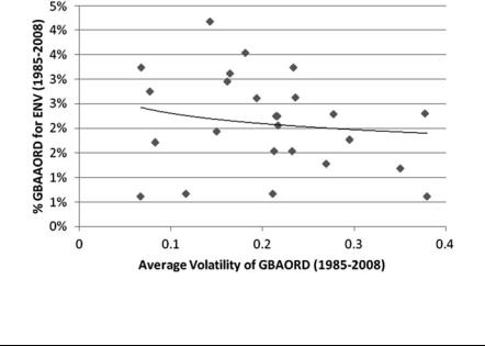
6 Implications of Policy Uncertainty for Innovation in Environmental Technologies. . . |
109 |
Fig. 6.1 Relationship between the level and volatility of ENV R&D spending
Table 6.1 Descriptive statistics
|
Number of |
|
|
|
|
Variable |
observations |
Mean |
Std. dev. |
Min |
Max |
|
|
|
|
|
|
Environmental patents |
422 |
78.06833 |
130.8575 |
0 |
537.331 |
TOTAL PATENTS (in ‘000s of |
422 |
3.954042 |
7.114198 |
0.010417 |
34.48414 |
patents) |
|
|
|
|
|
GBAORDENV (in millions of 2000 422 |
130.1552 |
169.6466 |
0.272 |
672.48 |
|
USD) |
|
|
|
|
|
POLICY UNCERTAINTY (lag) |
422 |
0.196477 |
0.141237 |
0.009715 |
0.809435 |
Table 6.2 Baseline results of the effect of policy uncertainty on innovation |
|
|
|||
|
|
|
|
|
|
|
(1) |
(2) |
|
(3) |
|
|
|
|
|
||
TOTAL PATENTS |
0.1085221*** |
0.0157791*** |
0.012334*** |
||
|
(0.0102444) |
(0.0036798) |
(0.0037922) |
||
GBAORDENV |
0.0030052*** |
0.0020716*** |
– |
|
|
|
(0.0002866) |
(0.0002344) |
– |
|
|
GBAORDENV (lag) |
– |
– |
|
0.0020853*** |
|
|
– |
– |
|
(0.0002536) |
|
POLICY UNCERTAINTY |
1.44427*** |
0.6286821*** |
0.6383595*** |
||
|
(0.3385673) |
(0.1577657) |
(0.1575273) |
||
Intercept |
2.954181*** |
4.407299*** |
4.506464*** |
||
|
(0.0834035) |
(0.1291679) |
(0.1318719) |
||
Country fixed effects |
No |
Yes |
|
Yes |
|
Number of obs. |
422 |
422 |
|
422 |
|
Log pseudolikelihood |
1,899.8567 |
1,447.43 |
1,449.6019 |
||
(Prob > Chi2) |
0 |
0 |
|
0 |
|
Note: (1) *** – significant at 1% level, ** – significant at 5% level, * – significant at 10% level; (2) Dependent variable is ENVPAT
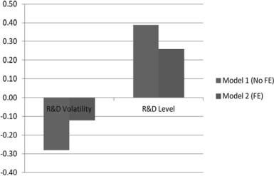
110 |
M. Kalamova et al. |
Fig. 6.2 Elasticities for the level and volatility of R&D spending
variable is positive and highly significant suggesting that patenting activity in the selected ‘environmental’ technologies is also explained by variation across countries and over time in patenting activity overall. In order to compare the relative magnitude of the coefficients, the elasticities have been calculated and are presented in Fig. 6.2. Thus, a 10% increase in policy uncertainty will cause a 1.2–2.8% decrease in environmental patent activity in the models with fixed effects (columns 2 and 3) and without fixed effects (column 1), respectively. At the same time, a 10% increase in government support for R&D will increase innovation by 2.6–3.9%.
Since the main explanatory variable in this study, POLICY UNCERTAINTY, is based on a government budget indicator (GBAORD), it is important to account for structural reforms occurring in the OECD economies which might have affected the reporting of public data. If we fail to account for potential breaks in the GBAORD series, the volatility of the uncertainty variable will be inflated. Indeed, we can identify several breaks in the GBAORD series, including the 1991 German reunification as well as the 1992 French economic reform to boost consumption and the record peak in surplus of the US federal budget in 2000. Therefore, in a subsequent step, we run the estimation on a reduced sample that accounts for structural breaks in the GBAORDENV variable and thus in the uncertainty measure. In general, the signs and significance levels of the explanatory variables remain the same as in the baseline estimation (except for the uncertainty measure in column 3), but the magnitudes of their estimated coefficients and elasticities change slightly. Thus, a 10% increase in policy uncertainty will cause a 0.6% (in the models with FEs) to 5.3% (without FEs) decrease in innovation activity whereas a 10% increase in GBAORDENV will increase innovation by 1.2–3.3%. Further robustness checks include the use of the logarithm of government R&D expenditures as well as their share in the country’s gross domestic product as explanatory variables. The regression analysis delivers the same qualitative results as in the baseline estimation (Table 6.3).
6 Implications of Policy Uncertainty for Innovation in Environmental Technologies. . . |
111 |
|||
Table 6.3 Tests of robustness |
|
|
|
|
|
|
|
|
|
|
(1) |
(2) |
(3) |
|
|
|
|
|
|
TOTAL PATENTS |
0.1281067*** |
0.0337766*** |
0.034552*** |
|
|
(0.0090737) |
(0.0073192) |
(0.0078704) |
|
GBAORDENV |
0.0026519*** |
0.001165*** |
– |
|
|
(0.0004066) |
(0.0003138) |
– |
|
GBAORDENV (lag) |
– |
– |
0.0010146*** |
|
|
– |
– |
(0.0003031) |
|
POLICY UNCERTAINTY |
3.007049*** |
0.3609491* |
0.3143938 |
|
|
(0.5914218) |
(0.2010824) |
(0.1997188) |
|
Intercept |
3.077275*** |
4.53315*** |
4.606643*** |
|
|
(0.1097179) |
(0.1347338) |
(0.1364057) |
|
Country fixed effects |
No |
Yes |
Yes |
|
Number of obs. |
295 |
295 |
295 |
|
Log pseudolikelihood |
1,298.3554 |
923.68148 |
926.60404 |
|
(Prob > Chi2) |
0 |
0 |
0 |
|
Note: (1) *** – significant at 1% level, ** – significant at 5% level, * – significant at 10% level; (2) Dependent variable is ENVPAT
6.5Conclusions and Policy Implications
Uncertainty associated with a country’s environmental policy – whether in terms of stringency, timing, nature or durability – will result in less innovation in environmental technologies. It may also bend the direction of innovation in a suboptimal manner. Since the planning horizon for investments in innovation is particularly long and the risk of being left with stranded assets is great, such investment decisions are likely to be significantly affected by policy uncertainty. The consequences can be manifold and include reduced and distorted investment in environmental R&D, delayed retirement of older facilities, suboptimal technology adoption choices and increased emission rates. Conversely, the more predictable a policy regime is, the more likely innovation is to take place and the more likely that this innovation will be directed in an optimal manner. This implies that governments should behave in a predictable manner if they wish to induce innovations that achieve environmental objectives at lower cost. Frequently changing policy conditions come at a cost. Uncertain signals give investors strong incentives to postpone investments, including the risky investments which lead to innovation. There is an advantage to ‘waiting’ until the policy dust settles. As such, by adding to the risk that investors face in the market, policy uncertainty can serve as a ‘brake’ on innovation, both in terms of technology invention and adoption. It is important to note that changing the policy parameters does not necessarily provide more uncertainty to investors as long as this is done in a predictable manner (e.g. periodic adjustments made in response to market developments). This implies that governments have an interest to behave in a predictable manner if they wish to induce innovations that achieve environmental objectives at lower cost. Moreover, these effects of policy uncertainty can be long-lived, stretching well beyond the
112 |
M. Kalamova et al. |
period of uncertainty, since future investment decisions will be affected by the credibility of signals given by policymakers in the past. A history of abrupt policy changes can discourage future investment long after the period of uncertainty has passed. Credibility is hard-won. However, it should be recognised that in some cases policy uncertainty can arise from the acquisition of new information. Damages may be higher or lower than initially foreseen, encouraging the use of more or less stringent policies. Similarly, abatement costs may be higher or lower than initially foreseen. In such cases, there is a trade-off between changing environmental objectives to reflect the new information and keeping incentives constant in order to reduce uncertainty. One possibility for mitigating the impacts of such trade-offs on the predictability of the policy signal is to design environmental policy in a manner that such ‘exogenous’ sources of uncertainty are explicitly built in alongside other policy parameters.
Appendix
IPC classes for environmental technologies
A.1. Air pollution abatement |
|
Filters or filtering processes specially modified for separating dispersed |
B01D46 |
particles from gases or vapours |
|
Separating dispersed particles from gases, air or vapours by liquid as |
B01D47 |
separating agent |
|
Separating dispersed particles from gases, air or vapours by other |
B01D49 |
methods |
|
Combinations of devices for separating particles from gases or vapours |
B01D50 |
Auxiliary pretreatment of gases or vapours to be cleaned from dispersed |
B01D51 |
particles |
|
Chemical or biological purification of waste gases |
B01D53/34-72 |
Separating dispersed particles from gases or vapour, e.g. air, by |
B03C3 |
electrostatic effect |
|
Use of additives to fuels or fires for particular purposes for reducing |
C10L10/02 |
smoke development |
|
Use of additives to fuels or fires for particular purposes for facilitating |
C10L10/06 |
soot removal |
|
Blast furnaces; dust arresters |
C21B7/22 |
Manufacture of carbon steel, e.g. plain mild steel, medium carbon steel |
C21C5/38 |
or cast steel; removal of waste gases or dust |
|
Exhaust or silencing apparatus having means for purifying or rendering |
F01N3 |
innocuous |
|
Exhaust or silencing apparatus combined or associated with devices |
F01N5 |
profiting by exhaust energy |
|
Exhaust or silencing apparatus, or parts thereof |
F01N7 |
Electrical control of exhaust gas treating apparatus |
F01N9 |
Combustion apparatus characterised by means for returning flue gases to |
F23B80 |
the combustion chamber or to the combustion zone |
|
Combustion apparatus characterised by arrangements for returning |
F23C9 |
combustion products or flue gases to the combustion chamber |
|
6 Implications of Policy Uncertainty for Innovation in Environmental Technologies. . . |
113 |
|
Incinerators or other apparatus specially adapted for consuming waste |
F23G7/06 |
|
gases or noxious gases |
|
|
Arrangements of devices for treating smoke or fumes of purifiers, e.g. |
F23J15 |
|
for removing noxious material |
|
|
Shaft or like vertical or substantially vertical furnaces; arrangements of |
F27B1/18 |
|
dust collectors |
|
|
A.2. Water pollution abatement |
|
|
Arrangements of installations for treating wastewater or sewage |
B63J4 |
|
Treatment of water, wastewater, sewage or sludge |
C02F |
|
Fertilisers from wastewater, sewage sludge, sea slime, ooze or similar |
C05F7 |
|
masses |
|
|
Chemistry; materials for treating liquid pollutants, e.g. oil, gasoline, fat |
C09K3/32 |
|
Devices for cleaning or keeping clear the surface of open water from oil |
E02B15/04-06 |
|
or like floating materials by separating or removing these materials; |
|
|
barriers therefore |
|
|
Cleaning or keeping clear the surface of open water; devices for |
E02B15/10 |
|
removing the material from the surface |
|
|
Methods or installations for obtaining or collecting drinking water or tap |
E03B3 |
|
water; rain, surface or groundwater |
|
|
Plumbing installations for wastewater |
E03C1/12 |
|
Sewers – cesspools |
E03F |
|
A.3. Waste management |
|
|
A.3.1. Solid waste collection |
|
|
Street cleaning; removing undesirable matter, e.g. rubbish, from the |
E01H15 |
|
land, not otherwise provided for |
|
|
Transporting; gathering or removal of domestic or like refuse |
B65F |
|
A.3.2. Material recovery, recycling and reuse |
|
|
Animal feeding – stuffs from distillers’ or brewers’ waste; waste |
A23K1/06-10 |
|
products of dairy plant; meat, fish or bones; kitchen waste |
|
|
Footwear made of rubber waste |
A43B1/12 |
|
Heels or top pieces made of rubber waste |
A43B21/14 |
|
Separating solid materials; general arrangement of separating plant |
B03B9/06 |
|
specially adapted for refuse |
|
|
Manufacture of articles from scrap or waste metal particles |
B22F8 |
|
Preparing material; recycling the material |
B29B7/66 |
|
Recovery of plastics or other constituents of waste material containing |
B29B17 |
|
plastics |
|
|
Presses specially adapted for consolidating scrap metal or for |
B30B9/32 |
|
compacting used cars |
|
|
Systematic disassembly of vehicles for recovery of salvageable |
B62D67 |
|
components, e.g. for recycling |
|
|
Stripping waste material from cores or formers, e.g. to permit their reuse |
B65H73 |
|
Applications of disintegrable, dissolvable or edible materials |
B65D65/46 |
|
Compacting the glass batches, e.g. pelletising |
C03B1/02 |
|
Glass batch composition – containing silicates, e.g. cullet |
C03C6/02 |
|
Glass batch composition – containing pellets or agglomerates |
C03C6/08 |
|
Hydraulic cements from oil shales, residues or waste other than slag |
C04B7/24-30 |
|
Calcium sulphate cements starting from phosphogypsum or from waste, |
C04B11/26 |
|
e.g. purification products of smoke |
|
|
Use of agglomerated or waste materials or refuse as fillers for mortars, |
C04B18/04-10 |
|
concrete or artificial stone; waste materials or refuse |
|
|

114
Claywares; waste materials or refuse
Recovery or working up of waste materials (plastics) Luminescent, e.g. electroluminescent, chemiluminescent, materials;
recovery of luminescent materials
Working up used lubricants to recover useful products
Working up raw materials other than ores, e.g. scrap, to produce nonferrous metals or compounds thereof
Obtaining zinc or zinc oxide; from muffle furnace residues; from metallic residues or scraps
Obtaining tin from scrap, especially tin scrap
Textiles; disintegrating fibre-containing articles to obtain fibres for reuse Papermaking; fibrous raw materials or their mechanical treatment using
waste paper
Papermaking; fibrous raw materials or their mechanical treatment; defibrating by other means of waste paper
Papermaking; other processes for obtaining cellulose; working up waste paper
Papermaking; pulping; non-fibrous material added to the pulp; waste products
Apparatus or processes for salvaging material from electric cables Recovery of material from discharge tubes or lamps
Reclaiming serviceable parts of waste cells or batteries Reclaiming serviceable parts of waste accumulators
A.3.3. Fertilisers from waste
Fertilisers made from animal corpses or parts thereof
Fertilisers from distillery wastes, molasses, vinasses, sugar plant, or similar wastes or residues
Fertilisers from waste water, sewage sludge, sea slime, ooze or similar masses
Fertilisers from household or town refuse
Preparation of fertilisers characterised by the composting step
A.3.4. Incineration and energy recovery
Solid fuels essentially based on materials of non-mineral origin; on sewage, house or town refuse; on industrial residues or waste materials
Cremation furnaces; incineration of waste; incinerator constructions; details, accessories or control therefore
Cremation furnaces; incinerators or other apparatus specially adapted for consuming specific waste or low-grade fuels
A.3.6. Waste management – not elsewhere classified
Disposal of solid waste
Production of liquid hydrocarbon mixtures from rubber or rubber waste Medical or veterinary science; disinfection or sterilising methods
specially adapted for refuse
A.4. Soil remediation
Reclamation of contaminated soil
A.5. Environmental monitoring
Monitoring or diagnostic devices for exhaust gas treatment apparatus Alarms responsive to a single specified undesired or abnormal condition
and not otherwise provided for, e.g. pollution alarms; toxics
M. Kalamova et al.
C04B33/132
C08J11
C09K11/01
C10M175
C22B7
C22B19/28-30
C22B25/06
D01G11
D21B1/08-10
D21B1/32
D21C5/02
D21H17/01
H01B 15/00
H01J 9/52
H01M 6/52
H01M 10/54
C05F1
C05F5
C05F7
C05F9
C05F17
C10L5/46-48
F23G5
F23G7
B09B
C10G1/10
A61L11
B09C
F01N11 G08B21/12-14
6 Implications of Policy Uncertainty for Innovation in Environmental Technologies. . . |
115 |
References
Aizenman, J., & Marion, N. P. (1993). Policy uncertainty, persistence and growth. Review of International Economics, 1(2), 145–163.
Baker, E., & Adu-Bonnah, K. (2008). Investment in risky R&D programs in the face of climate uncertainty. Energy Economics, 30, 465–486.
Baker, E., & Shittu, E. (2006). Profit-maximizing R&D in response to a random carbon tax.
Resource and Energy Economics, 28, 160–180.
Barradale, M. J. (2008). Impact of policy uncertainty on renewable energy investment: Wind power and PTC (Working Paper 08-003). US Association for Energy Economics.
Bloom, N., & Van Reenen, J. (2002). Patents, real options and firm performance. The Economic Journal, 112, C97–C116.
Bohm, M. C., Herzog, H. J., Parsons, J. E., & Sekar, R. C. (2007). Capture-ready coal plants: Options, technologies and economics. International Journal of Greenhouse Gas Control, 1, 113–120.
Brunnermeier, S. B., & Cohen, M. A. (2003). Determinants of environmental innovation in US manufacturing industries. Journal of Environmental Economics and Management, 45, 278–293.
Burtraw, D., & Palmer, K. (2004). SO2 Cap-and-trade program in the United States. In W. Harrington, R. Morgenstern, & T. Sterner (Eds.), Choosing environmental policy: Comparing instruments and outcomes in the United States and Europe. Washington, DC: RFF Press.
Cameron, A. C., & Trivedi, P. K. (1998). Regression analysis of count data. Cambridge: Cambridge University Press.
Czarnitzki, D., & Toole, A. A. (2011). Patent protection, market uncertainty, and R&D investment.
The Review of Economics and Statistics, 93(1), 147–159.
Dernis, H., Guellec, D., & van Pottelsberghe de la Potterie, B. (2001). Using patent counts for crosscountry comparisons of technology output. STI mimeo, Paris: Organisation for Economic Co-operation and Development. http://www.oecd.org/dataoecd/26/11/21682515.pdf
Dixit, A. K., & Pindyck, R. S. (1994). Investment under uncertainty. Princeton: Princeton University Press.
Farzin, Y. H., & Kort, P. M. (2000). Pollution abatement investment when environmental regulation is uncertain. Journal of Public Economic Theory., 2(2), 183–212.
Fuss, S., Szolgayova, J., Obersteiner, M., & Gusti, M. (2008). Investment under market and climate policy uncertainty. Applied Energy, 85, 708–721.
Goel, R. K., & Ram, R. (2001). Irreversibility of R&D investment and the adverse effect of uncertainty: Evidence from the OECD countries. Economics Letters, 71(2), 287–291.
Griliches, Z. (1990). Patent statistics as economic indicators: A survey. Journal of Economic Literature, 28(4), 1661–1707.
Hausman, J., Hall, B. H., & Griliches, Z. (1984). Econometric models for count data with an application to the patents-R&D relationship. Econometrica, 52, 909–938.
Hicks, J. R. (1932). The theory of wages. London: Macmillan.
Isik, M. (2004). Incentives for technology adoption under environmental policy uncertainty: Implications for green payment programs. Environmental and Resource Economics, 27, 247–263.
Johnstone, N., Hascic, I., & Kalamova, M. (2010). Environmental policy characteristics and technological innovation. Economia Politica, 2, 277–301.
Johnstone, N., Hasˇcˇicˇ, I., Poirier, J., Hemar, M., & Michel, C. (2012). Environmental Policy Stringency and Technological Innovation: Evidence from Survey Data and Patent Counts.
Applied Economics, 44, 2157–2170.
Lanjouw, J. O., & Mody, A. (1996). Innovation and the international diffusion of environmentally responsive technology. Research Policy, 25(5), 49–571.
116 |
M. Kalamova et al. |
Lofgren,¨ |
˚ |
A., Millock, K., & Nauges, C. (2008). The effect of uncertainty on pollution abatement |
investments: Measuring hurdle rates for Swedish industry. Resource and Energy Economics, 30, 475–491.
Maddala, G. S. (1983). Limited-dependent and qualitative variables in econometrics. Cambridge: Cambridge University Press.
Maynard, L. J., & Shortle, J. S. (2001). Determinants of cleaner technology investments in the U.S. bleached kraft pulp industry. Land Economics, 77(4), 561–576.
OECD. (2002). Frascati manual 2002: Proposed standard practice for surveys on research and experimental development. Paris: OECD.
OECD. (2009). OECD patent statistics manual. Paris: OECD.
Pindyck, R. S. (1991a). Irreversibility and the explanation of investment behavior. In D. Lund & B. Oksendal (Eds.), Stochastic models and option values. New York/Amsterdam: Elsevier Science Publishers/North-Holland.
Pindyck, R. S. (1991b). Irreversibility, uncertainty, and investment. Journal of Economic Literature, 29, 1110–1152.
Pindyck, R. S. (2007). Uncertainty in environmental economics. Review of Environmental Economics and Policy, 1, 45–65.
Purvis, A., Boggess, W. G., Moss, C. B., & Holt, J. (1995). Technology adoption decisions under irreversibility and uncertainty: An ‘ex ante’ approach. American Journal of Agricultural Economics, 77(3), 541–551.
Reinelt, P., & Keith, D. (2007). Carbon capture retrofits and the cost of regulatory uncertainty.
Energy Journal, 28(4), 101–128.
Rodrik, D. (1991). Policy uncertainty and private investment in developing countries. Journal of Development Economics, 36, 229–242.
So¨derholm, P., Ek, K., & Pettersson, M. (2007). Wind power development in Sweden: Global policies and local obstacles. Renewable and Sustainable Energy Reviews, 11, 365–400.
Wiser, R. H., & Pickle, S. J. (1998). Financing investments in renewable energy: The impacts of policy design. Renewable and Sustainable Energy Reviews, 2, 361–386.
Xepapadeas, A. (2001). Environmental policy and firm behavior: Abatement investment and location decisions under uncertainty and irreversibility. In C. Carraro & G. E. Metcalfe (Eds.), Behavioral and distributional effects of environmental policy (pp. 281–308). Chicago: University of Chicago Press.
Yang, M., Blyth, W., Bradley, R., Bunn, D., Clarke, C., & Wilson, T. (2008). Evaluating the power investment options with uncertainty in climate policy. Energy Economics, 30, 1933–1950.

Chapter 7
Eco-Activity and Innovativeness: What Is Their Relation to Environmental Performance
in Consumer Firms and Industrial Firms?
Nicoline Oehme and Rene´ Kemp
Abstract This chapter examines the link between environmental performance, corporate social performance and innovativeness for consumer and industrial firms, using company data on R&D, environmental and corporate social performance from the Kinder, Lydenberg and Domini (KLD) database for US-based firms. We find empirically that during the period from 1999 to 2008, there has been an increase in environmental action, especially since 2004. A positive correlation is found to exist between environmental and non-environmental social performance in many dimensions and a positive but weak link between environmental performance and R&D per employee or unit of sales. This chapter shows that there is a difference between consumer and industrial firms in terms of the evolution of eco-activities and environmental impact. Contrary to what we expected, industrial firms undertook more product-related eco-activities than consumer firms. Industrial firms also showed a greater increase in process-related eco-activity. The increase in ecoactivity went with an increase in eco-impact in both company types, suggesting that environmental action did not arrest environmental degradation overall.
Keywords Eco-activity • Environmental performance • Consumer firms • Industrial firms • Innovativeness • Social performance
N. Oehme
mgm consulting partners GmbH, Holla¨ndischer Brook 2, 20457 Hamburg, Germany e-mail: n.oehme@googlemail.com
R. Kemp (*)
UNU-MERIT and ICIS, Maastricht University, Keizer Karelplein 19, Maastricht, The Netherlands e-mail: r.kemp@maastrichtuniversity.nl
V. Costantini and M. Mazzanti (eds.), The Dynamics of Environmental |
117 |
and Economic Systems: Innovation, Environmental Policy and Competitiveness,
DOI 10.1007/978-94-007-5089-0_7, # Springer Science+Business Media Dordrecht 2013

118 |
N. Oehme and R. Kemp |
7.1Introduction
This chapter tests a number of propositions about consumer and industrial firms’ environmental behaviour and performance, using longitudinal data for US companies. We also examine the link between environmental performance and the non-environmental part of corporate social performance. The novelty of this chapter is that we examine these links using panel data over an extended period for consumer and industrial firms. This study makes a distinction between eco-activity and eco-impact. Whereas the first expresses what firms do in order to decrease their environmental harm, the latter represents firms’ environmental harm. These two elements are not necessarily complementary since firms may very well increase or decrease both elements at the same time. The first two propositions are:
•Firms’ eco-activity has increased over the past 10 years (H1a).
•Firms’ eco-impact has not increased over the past 10 years (H1b).
We expect companies’ eco-activity to have increased over the past 10 years because of stricter environmental policy, greater attention to climate change, the need to move away from fossil fuels, rising demand for green products and companies accepting environmental responsibility, topics that are widely believed to have increased in the period 1999–2008. In the academic literature, it has been stated that environmental performance is becoming increasingly important and firms should engage in environmental protection activities through innovation (Hart 1995, 2007; Senge et al. 2008; Hall and Vredenburg 2003; Florida 1996; Porter and van der Linde 1995; Gladwin et al. 1995; Shrivastava 1995; Stead and Stead 1994).
The second set of propositions is:
•Innovativeness is positively related to eco-activity in the most recent years (H2a).
•Innovativeness is positively related to improved eco-impact in the most recent years1 (H2b).
We expect innovation to be positively related to eco-activity at least in more recent years, and we also expect this to be reflected in eco-impact which should have improved. We are not sure whether firms managed to achieve an absolute improvement in eco-impact, but we do expect a relative improvement due to innovation.
As third point, other tested propositions are:
•Innovativeness is positively related to product eco-activity (H3a).
•Innovativeness is positively related to improved product eco-impact (H3b).
•Innovativeness is positively related to process eco-activity (H3c).
•Innovativeness is positively related to improved process eco-impact (H3d).
1 By improved eco-impact, we mean that the level of pollution and hazardous waste is reduced.
7 Eco-Activity and Innovativeness: What Is Their Relation. . . |
119 |
We expect innovativeness to be positively related to product and process eco-activity and to product and process eco-impact. We are less sure that we will find a positive relation between innovation and eco-impact since eco-impact depends above all on the scale and type of products produced.
Then, as fourth set of propositions, we focus on:
•Over the past 10 years, industrial firms’ eco-activity has increased more than that of consumer firms (H4a).
•Over the past 10 years, industrial firms’ eco-impact has increased less or decreased more than that of consumer firms (H4b).
The argument for expecting industrial firms to be more active in eco-activity is that they are generally more polluting and thus more subject to regulations than consumer firms. Of the various drivers, regulations are identified as the most powerful driver for environmental performance (Bansal and Roth 2000; Fineman and Clarke 1996; Florida 1996). As a result, we expect the eco-impact from industrial firms to have improved more or worsened less than that of consumer firms.
The fifth set of empirical tests is:
•Consumer firms show a higher product than process-related eco-activity (H5a).
•Consumer firms show a lower product than process-related eco-impact (H5b).
We expect eco-activities of consumer firms to be more focused on product ecoactivities than on processes, which are reflected in the eco-impact from products that have improved more than that of processes. This is because product-related eco-activities are more visible to the consumer when buying a product.
We also test whether:
•Industrial firms show a higher process than product-related eco-activity (H6a).
•Industrial firms show a lower process than product-related eco-impact (H6b).
For industrial firms, we expect innovation to be more focused on process than on product, i.e. the mirror image for consumer firms.
Some tests regard CSR issues:
•Non-eco corporate social strengths are positively related to eco-activity (H7a).
•Non-eco corporate social concerns are positively related to eco-impact (H7b).
We in fact do expect eco-activity and eco-impact to be positively correlated with non-environmental corporate social responsibility activities. CSR companies can be expected to take on responsibility for both environmental and nonenvironmental issues as a matter of ethos and because there is a reputation effect at stake. If companies perform badly in one social performance category, perceptions of the entire social performance suffer (Liston-Heyes and Ceton 2008).
Finally, we test whether:
•Non-eco corporate social strengths are a better predictor for eco-activity than innovativeness and firm type (H8a).
120 |
N. Oehme and R. Kemp |
•Non-eco corporate social concerns are a better predictor for eco-impact than innovativeness and firm type (H8b).
Non-eco CSR action is believed to be a better predictor for eco-activity than innovativeness and firm type. This is expected to hold true for the entire period.
To conclude, this chapter examines firms’ environmental performance development over time in relation to its innovativeness for consumer and industrial firms. Different aspects of environmental performance are highlighted.
7.2Sample
The sample consists of business-to-business (B2B) companies and business- to-consumer (B2C) companies. B2B and B2C companies are called industrial firms and consumer firms, respectively. The SIC code was used to include only producing industries that potentially have both consumers and firms as customers. Consequently, the manufacturing and wholesale trade industries are included. These are firms with SIC codes 2000 to 3999 and 5000 to 5199, respectively. We used information from companies included in the KLD database. The KLD agency is an independent institution based in the USA that gives points to firms based on their social performance. The rating agency merely monitors listed US-based corporations. Consequently, only larger US-American companies are included in this study. The KLD agency initially started in 1990 by examining the social performances of all companies in the S&P 500® Index and Domini 400 Social SM Index (KLD Research and Analytics, Inc. 2010). The number of companies in the database grew from 650 firms in 1991 to 3,100 firms in 2003 (KLD Research and Analytics, Inc. 2010). Since 2003, no further expansions have taken place. As this study is about the firms’ change in time, only companies whose data is available from 1999 to 2008 are included in the sample. Moreover, retailers are excluded. As a result, the sample for this study consists of 195 firms.
Experts with various backgrounds assess the firms annually by using public sources and questionnaires filled in by the firms themselves or by non-governmental organizations (KLD 2007). The use of independent experts guards against inflated claims about performance (Graves and Waddock 1994; Liston-Heyes and Ceton 2008; Waddock and Graves 1997). The assessment is based on objective information as much as possible (Waddock and Graves 1997). For instance, regulatory problems are rated as dollars paid for fines (Waddock and Graves 1997). Since the criteria are applied similarly for each company in each year, the dataset gives consistent ratings (Waddock and Graves 1997; Harrison and Freeman 1999) over time and across industries. In general, the KLD dataset has been proven to give valid results (Sharfman 1996) and found to indeed measure corporate social and environmental performance (Chatterji et al. 2009; Harrison and Freeman 1999). The KLD rating of social corporate performance covers human rights, controversial business involvement, employee relations and environmental aspects. The latter is
7 Eco-Activity and Innovativeness: What Is Their Relation. . . |
121 |
Table 7.1 KLD rating categories |
|
|
|
Strengths (eco-activity) |
Concerns (eco-impact) |
Clean energy |
Climate change |
Beneficial products and services |
Ozone-depleting chemicals |
|
Agricultural chemicals |
Pollution prevention |
Hazardous waste |
Recycling |
Regulatory problems |
Management system (since 2006) |
Substantial emissions |
Other strengths |
Other concerns |
|
|
the focus of this study. The environmental performance consists of so-called strengths and concerns (Table 7.1) of which specific aspects are rated.
The KDL agency uses the terms strengths and concerns where strengths mean that the company assessed performs well on the specific environmental aspect, whereas concerns are environment-harming issues for which further action is needed. The terms are somewhat misleading. Whenever a firm has strengths in this dataset, it does not mean that the company is good for the environment. To avoid confusion, in this chapter, the term eco-activity is used for strengths and (negative) eco-impact for concerns.
Each category is rated binary. If the assessment indicated that a company fulfils certain criteria for a category (strengths or concerns), it is indicated by value ‘one’; 0 denotes neutrality (KLD Research and Analytics, Inc. 2010). For example, a company that recycles a substantial part of its waste has a ‘one’ in the category Recycling. If it had to pay fines for environmental issues, this will be shown in the category Regulatory Problems as a ‘one’. Likewise, no fines will result in a 0. It is important to note that if a firm shows the same activity or impact every year, they are also rated each year in the same way. The dataset further aggregates data in that for environmental performance, all elements of strengths (here activity) and of concerns (impact) are added separately, giving each category the same weight. Giving equal weights does not fully represent the reality (Graves and Waddock 1994), but weighting each category according to its importance would require detailed understanding and theoretical background of these measures (Hillman and Keim 2001). This is too complex if not impossible for a study about various industries such as this one. Some studies further consolidate the data by subtracting the number of concerns from the strengths to have one indicator for each company only (Turban and Greening 1996; Hillman and Keim 2001; Waddock and Graves 1997). This is a problematic method since it has been shown that both correlate (Chatterji et al. 2009). Consolidating the two values would give similar results for companies that are rather neutral and companies that have high ratings in both eco-activity and impact. This reduces the variation of the data (Sharfman and Fernando 2008), and some further insights are lost. Since this procedure is questionable, it is not applied in this study. In this study, all elements of eco-activity and impact are added separately giving each criterion the same weight. However, these two measures are not further combined in any way.
122 |
N. Oehme and R. Kemp |
Corporate social performance indicators are also published by the KLD agency. They include community, corporate governance, diversity, employee relations, human rights and product-related factors. In terms of corporate social performance, the terms strengths and concerns are considered appropriate. Strengths and concerns are collected for the same period of time for all categories.
Companies in the sample were classified as industrial or consumer firms using information publicly available such as companies’ homepages or annual reports. Usually, the sector of each company indicates whether it sells mainly to firms or to consumers. Whenever a company serves both markets, annual reports and its financial information were used to determine the customer base. When no clear focus could be established on either side or serving firms and consumers was explicitly mentioned, it was classified as ‘serving both types of customers’. This classification gives three main groups: 94 industrial and 41 consumer firms and 60 that produce for both types of customers. It is assumed that the customer base companies did not change during the analysed period. During this search, retailers were excluded as mentioned above. A student randomly checked and agreed with the classifications.
For measuring innovation, we used R&D expenditure. R&D expenditure is a commonly used innovation indicator, together with patents (Kleinknecht et al. 2002; Hagedoorn and Cloodt 2003). For this study, patent and patent citation is not sensible to use because patenting behaviour varies between industries (Shane and Toby 2002). New product announcement however only includes products and no process changes. The R&D indicator does not suffer from this as R&D is used to improve products and processes. Certainly, R&D also varies per industry since some industries are more research based such as pharmaceutical industries. However, if the theory in this study holds, then the companies in R&D intensive industries should also perform increasingly better in environmental terms. Thus, R&D expenditure is regarded to be appropriate for this study since it indicates the potential to change. For companies in the sample, the R&D expenses for the period 1994–2008 were collected from the Standard & Poor’s Compustat dataset. Here, a longer period of time was chosen since R&D expenditure potentially requires some time to take effect. In order to compare the R&D expenditure over time, this expenditure was adjusted for inflation with data given for each time period (Financial Trend Forecaster 2010). To do this, 1994 serves as a base year. For company size, we used information about turnover and number of employees for each firm for each year, collected from the same database. This divides the R&D expenditure by the number of employee or turnover in order to have two different relative measures of innovativeness.
7.3Analysis of Environmental Performance and Innovativeness
First, the general development of eco-activity and eco-impact is examined (Fig. 7.1).
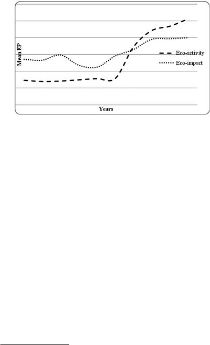
7 Eco-Activity and Innovativeness: What Is Their Relation. . . |
123 |
Fig. 7.1 Development of eco-activity and impact—all firms (1999–2008)
Eco-activity remains stable until year 2004, and then it rapidly increases with a modest flattening since 2006. Eco-impact shows a more irregular pattern. It is reasonably stable from 1999 to 2001 and then decreases for 2 years, followed by an increase up to 2006. In 2007 and 2008, it stabilizes again. Since 2004 and 2005, activity is outperforming eco-impact.
The development is also tested statistically by paired sample t-tests for the overall difference between 1999 and 2008 for eco-activity and impact. The overall increase in eco-activity is significant with p < 0.01 (M ¼ 0.512, SD ¼ 0.925, t (40) ¼ 3.545). Thus, H1a can be supported. The overall increase in eco-impact is also significant with p ¼ 0.000 (M ¼ 0.122, SD ¼ 0.781, t(40) ¼ 1.000). This is contrary to the prediction. Consequently, H1b cannot be supported.
In order to test the relation between innovativeness and eco-activity and impact, Spearman’s rank correlations are applied. First, the correlation for innovativeness and eco-activity is examined and indicates that no combination is significant (Tables 7.7 and 7.8 in Appendix A). This means that H2a cannot be supported due to the lack of significant correlation in the most recent years. The relation between innovativeness and eco-impact has more significant relations, and all of them are negative. The eco-impact for 2006 correlates with innovativeness from 1994 to 1998 as well as with 2000 and 2001 with at least p < 0.05, eco-impact of 2007 correlates with innovativeness of years 1994 until 2004 and 2007 (1994 until 1997 and 2000, p < 0.01, for all other p < 0.05) and the eco-impact of 2008 is correlated with innovativeness of 1994 until 2003 (1994–1997; p < 0.01, all other p < 0.05).2 The strong correlation in the later years is a strong support for H2b. To add, it reveals that some time has to pass for R&D expenditure to have any
2 Here, innovativeness is R&D expenditure per employee. For R&D expenditure per turnover, the numbers vary, but the underlying result remains the same.
124 |
|
|
|
N. Oehme and R. Kemp |
Table 7.2 Allocation of product and process categories |
|
|||
|
|
|
|
|
Products |
|
Process |
|
|
|
|
|
|
|
Eco-activity |
Eco-impact |
Eco-activity |
Eco-impact |
|
Green product |
Climate change |
Pollution prevention |
Hazardous waste |
|
|
Ozone-depleting chemicals |
|
Recycling |
Substantial emissions |
|
Agricultural chemicals |
|
|
|
|
|
|
|
|
correlation with eco-activity or eco-impact. Although there are some exceptions, most of the time, there is a time lag between R&D spending and eco-impact of at least 3 years.
We also examined whether the link between innovation and eco-activity and eco-impact differs between product and process practices of environmental performance. The elements of environmental performance are classified into four groups according to the descriptions given by KLD (KLD Research and Analytics, Inc. 2010). These groups are product-related eco-activity, product-related eco-impact, processrelated eco-activity and process-related eco-impact. Table 7.2 shows the allocation of the elements. Product categories include all elements that can be directly related to the product. Process-related elements are those that take place during or are caused by the process of manufacturing the product. KLD categories clean energy and regulatory problems cannot be clearly allocated to either process or product because they can be related to both, product or process, according to the description by KLD (2010). Therefore, they are not included in any analysis of process and product performances. The allocation does not result in same-sized categories. Since the categories are compared directly during the analyses, the average for all measures per category is used.
For the relation between innovativeness and product and process practices, a Spearman correlation analysis is once again applied. No correlation at all can be found (Tables 7.9, 7.10, 7.11 and 7.12 in Appendix B). Although not significant, most of the correlations between innovativeness and product eco-activity are negative; for process eco-activity, most of the correlations were negative from 1999 to 2001. Since then, many are positive. The relation between innovativeness and product-related eco-impact is increasingly negative, and process-related ecoimpact and innovativeness have always been negatively related. Most of these trends would not support the hypotheses even if they were significant. Therefore, H3a–H3d cannot be supported.
Before analysing whether industrial and consumer firms act upon eco-activity or impact to different extents, their separate development is assessed. The development of consumer firms’ eco-activity and impact looks similar to the figure for all firms (Fig. 7.2) except that the mean eco-impact remains moderately stable over time (Fig. 7.3). Here again, in the most recent years, eco-activity has outperformed eco-impact.
Industrial firms’ eco-activity remained very stable until 2004, and since then, it has increased significantly (Fig. 7.3). Eco-impact first shows a minor increase, followed by a decrease for two years and then another eco-impact increase.
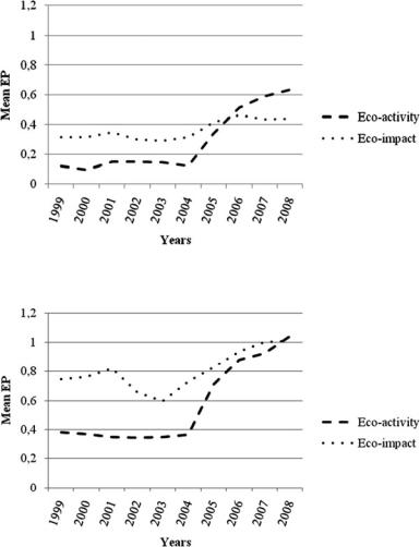
7 Eco-Activity and Innovativeness: What Is Their Relation. . . |
125 |
Fig. 7.2 Development of eco-activity and impact—consumer firms (1999–2008)
Fig. 7.3 Development of eco-activity and impact—industrial firms (1999–2008)
Eco-impact has worsened since 2004 in the face of an increase in eco-activity. The eco-impact mean is higher than that of eco-activity for all years, except for the year 2008 when eco-activity is marginally higher.
In order to test whether industrial or consumer firms have a larger increase in terms of eco-activity or impact, the difference between 1999 and 2008 was calculated for eco-activity and impact for each firm. With these variables, two independent sample t-tests are conducted. The test presents the following: the eco-activity increase in consumer firms (M ¼ 0.5122, SD ¼ 0.92526) and industrial firms (M ¼ 0.6596, SD ¼ 1.01126) does not differ significantly (t(133) ¼ 0.798, p ¼ 0.426). Neither does the increase in eco-impact per firm type significant
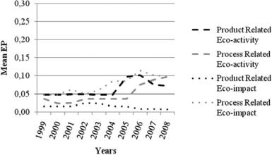
126 |
N. Oehme and R. Kemp |
Fig. 7.4 Product and process eco-activity and impact—consumer firms (1999–2008)
(consumer firms: M ¼ 0.122, SD ¼ 0.78087; |
industrial firms: |
M ¼ 0.266, |
SD ¼ 0.86975; t(84.375) ¼ 0.951, p ¼ 0.364). |
Therefore, no |
significant |
differences in the development in general are found: H4a and H4b are not supported.
In the following section, we examine the relation between firm type and processand product-related environmental performance.
From 1999 until 2008, the practices of consumer firms diverged (Fig. 7.4). All practices are relatively close in 1999. While process-related eco-impact increased steadily over the examined period, product-related eco-activity increased abruptly in 2004 and process-related eco-activity in 2005. Since 2006, the means of processrelated eco-impact and product-related eco-activity decreased marginally again. In 2008, process-related eco-impact and eco-activity have very similar means which are slightly higher than that of product-related eco-activity. The mean of productrelated eco-impact is constantly close to zero. This figure shows many intersections but none with product-related eco-impact which is constantly fairly low.
Whether the practices differ significantly for consumer firms is tested in paired sample t-tests in order to compare product and process eco-activity as well as product and process eco-impact (Table 7.3). The tests show that there are hardly any significant differences. There is no significant difference at all between product- and process-related eco-activity. H5a is therefore not supported. On the contrary, H5b is supported since process eco-impact is significantly higher than product eco-impact from 2004 until 2008 (for 2004 p < 0.1, 2005 p < 0.05, 2006 p < 0.01 2007 and 2008 p < 0.05). This is mainly due to the increase in processrelated eco-impact. Product-related eco-impact stayed more or less constant during the entire period (it did not worsen).
If we consider the specific measures for process and product eco-activity, we find that the increase in process eco-activity is mainly due to the rise in recycling
7 Eco-Activity and Innovativeness: What Is Their Relation. . . |
|
|
127 |
||||
Table 7.3 Paired sample t-tests: product and process EP—consumer firms |
|
|
|||||
|
|
|
|
|
|
|
|
|
|
Paired |
|
|
|
|
|
|
|
differences |
|
t |
|
|
|
|
|
|
|
Std. |
|
Sig. |
|
|
Year |
Mean |
|
deviation |
df |
(2-tailed) |
|
Productand process-related eco- |
1999 |
0.012 |
0.262 |
0.298 |
40 |
0.767 |
|
activity |
2000 |
0.024 |
0.249 |
0.628 |
40 |
0.534 |
|
|
2001 |
0.025 |
0.252 |
0.628 |
39 |
0.534 |
|
|
2002 |
0.013 |
0.265 |
0.298 |
39 |
0.767 |
|
|
2003 |
0.012 |
0.262 |
0.298 |
40 |
0.767 |
|
|
2004 |
0.012 |
0.262 |
0.298 |
40 |
0.767 |
|
|
2005 |
0.061 |
0.255 |
1.532 |
40 |
0.133 |
|
|
2006 |
0.026 |
0.343 |
0.467 |
38 |
0.643 |
|
|
2007 |
0.013 |
0.314 |
0.255 |
38 |
0.800 |
|
|
2008 |
0.024 |
0.315 |
0.495 |
40 |
0.623 |
|
Productand process-related eco- |
1999 |
0.033 |
0.183 |
1.135 |
40 |
0.263 |
|
impact |
2000 |
0.033 |
0.183 |
1.135 |
40 |
0.263 |
|
|
|||||||
|
2001 |
0.046 |
0.210 |
1.380 |
39 |
0.176 |
|
|
2002 |
0.025 |
0.171 |
0.924 |
39 |
0.361 |
|
|
2003 |
0.037 |
0.185 |
1.270 |
40 |
0.212 |
|
|
2004 |
0.069 |
0.220 |
2.008 |
40 |
0.051 |
|
|
2005 |
0.069 |
0.201 |
2.206 |
40 |
0.033 |
|
|
2006 |
0.107 |
0.243 |
2.742 |
38 |
0.009 |
|
|
2007 |
0.094 |
0.235 |
2.498 |
38 |
0.017 |
|
|
2008 |
0.089 |
0.230 |
2.489 |
40 |
0.017 |
|
activities, especially since 2005. However, recycling can also be seen as a product activity. If we consider recycling a product activity, the measure for product ecoactivity has risen drastically since 2004 (Fig. 7.5). This would clearly support H5a.
Industrial firms have developed differently from consumer firms in the past 10 years in terms of applied practices. The means of product-related eco-impact as well as process-related eco-activity remained relatively stable and low (Fig. 7.6). The means of product-related eco-activity was almost constant until 2004 and then increased somewhat irregularly. The movement of process-related eco-impact is even more irregular, but in general, it shows an increase.
The development is tested with paired sample t-tests. The tests indicate that except for year 1999, eco-activity differs significantly for each year in that productrelated eco-activity is always higher than that of process-related eco-activity (with mostly p < 0.05, and only in 2000 p < 0.1). Thus, H6a cannot be supported. Even more so, it is seen to be the opposite of what was predicted. Processand product-related eco-impact differs significantly in all years (with p < 0.01), namely, process-related eco-impact is higher than product-related ones. Consequently, H6b cannot be supported either (Table 7.4).
Classifying recycling as a product-related eco-activity does not result in any major differences for the hypotheses for industrial firms (Fig. 7.7).
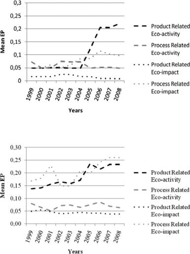
128 |
N. Oehme and R. Kemp |
Fig. 7.5 Product and process eco-activity and impact—consumer firms (recycling as productrelated) (1999–2008)
Fig. 7.6 Product and process eco-activity and impact—industrial firms (1999–2008)
7.4Analysis of Non-environmental Social and Environmental Performance
In order to test the relation between non-eco corporate social and environmental performance, all strengths of the different elements of corporate social performance, except environmental elements, are added. The same is repeated for concerns. Corporate social strengths and concerns increased fairly steadily during the period from 1999 until 2008 (Fig. 7.8) with strengths constantly higher than concerns.
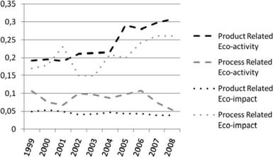
7 Eco-Activity and Innovativeness: What Is Their Relation. . . |
|
|
129 |
|||||
Table 7.4 Paired sample t-tests: product and process EP – industrial firms |
|
|
||||||
|
|
|
|
|
|
|
|
|
|
|
Paired |
|
|
|
|
|
|
|
|
differences |
|
t |
|
|
|
|
|
|
|
|
|
Std. |
|
Sig. |
|
|
|
Mean |
|
deviation |
df |
(2-tailed) |
|
|
Productand process-related |
1999 |
0.059 |
0.427 |
1.330 |
93 |
0.187 |
||
eco-activity |
2000 |
0.076 |
0.419 |
1.742 |
91 |
0.085 |
||
|
2001 |
0.107 |
0.416 |
2.420 |
88 |
0.018 |
||
|
2002 |
0.094 |
0.417 |
2.151 |
89 |
0.034 |
||
|
2003 |
0.085 |
0.399 |
2.067 |
93 |
0.042 |
||
|
2004 |
0.108 |
0.403 |
2.575 |
92 |
0.012 |
||
|
2005 |
0.161 |
0.455 |
3.415 |
92 |
0.001 |
||
|
2006 |
0.129 |
0.466 |
2.672 |
92 |
0.009 |
||
|
2007 |
0.165 |
0.477 |
3.349 |
93 |
0.001 |
||
|
2008 |
0.170 |
0.473 |
3.491 |
93 |
0.001 |
||
Productand process-related |
1999 |
0.121 |
0.277 |
4.221 |
93 |
0.000 |
||
eco-impact |
2000 |
0.125 |
0.269 |
4.455 |
91 |
0.000 |
||
|
||||||||
|
2001 |
0.182 |
0.310 |
5.520 |
88 |
0.000 |
||
|
2002 |
0.109 |
0.266 |
3.900 |
89 |
0.000 |
||
|
2003 |
0.106 |
0.277 |
3.718 |
93 |
0.000 |
||
|
2004 |
0.163 |
0.334 |
4.706 |
92 |
0.000 |
||
|
2005 |
0.156 |
0.318 |
4.723 |
92 |
0.000 |
||
|
2006 |
0.199 |
0.331 |
5.798 |
92 |
0.000 |
||
|
2007 |
0.222 |
0.349 |
6.150 |
93 |
0.000 |
||
|
2008 |
0.222 |
0.352 |
6.105 |
93 |
0.000 |
||
Fig. 7.7 Product and process eco-activity and impact—industrial firms (recycling as productrelated)

130 |
N. Oehme and R. Kemp |
Fig. 7.8 Development of corporate social performance (1999–2008)
Spearman rank-order correlation analyses are conducted for non-eco corporate social strengths and concerns in relation to eco-activity and impact, respectively. The correlation between eco-activity and non-eco corporate social strengths increases steadily. More precisely, since 2003, almost all eco-activity has been significantly correlated with non-eco corporate social strengths. Accordingly, H7a has been supported for eco-activity since 2003, but not for the previous period. Interestingly, every possible combination of eco-impact and non-eco corporate social strengths is correlated. Non-eco social corporate activities are associated with improved environmental performance in terms of reduced concerns. Hence, H7b is supported. In addition, non-eco corporate social concerns and eco-activity show numerous significant relations, especially since 2005.
Additionally, we tested whether there is a difference between firm types with respect to non-eco corporate social performance. Indeed, there is a difference for corporate social strengths, in that consumer firms show a significant better performance for all years, as expected. Corporate social concerns do not differ between firm types.
In order to know which of the three factors, innovativeness, firm type or non-eco corporate social performance, has the most predicting power for both parts of environmental performance, several regression analyses are conducted.3 For this, the classification of firm type is transformed to a scale, 1 being industrial firms and
3 Outliers were excluded in order to have a Mahalanobis distance below 13.82 (Pallant 2007). We also checked for multicollinearity in the explanatory variables and the normal distribution of the errors.
7 Eco-Activity and Innovativeness: What Is Their Relation. . . |
|
|
|
131 |
|||||||
Table 7.5 Regression for non-eco CSP, firm type and innovativeness |
|
|
|
||||||||
|
|
|
|
|
|
|
|
|
|
|
|
|
|
Model |
|
ANOVA |
Coefficients |
|
|
|
|
||
|
|
|
|
|
|
|
|
|
|
|
|
|
|
Adjusted R |
|
|
|
|
|
|
|
|
|
|
|
square |
|
df |
F |
Sig |
beta |
t |
Sig |
||
|
|
|
|
|
|
|
|
|
|
||
Eco-activity |
Firm type |
0.18 |
(3, 141) |
11.571 |
|
0.000 |
0.269 |
3.485 |
0.001 |
||
1999 |
Innovativeness |
|
|
|
|
|
|
|
0.149 |
1.926 |
0.056 |
|
|
|
|
|
|
|
|
||||
|
1994 |
|
|
|
|
|
|
|
|
|
|
|
Non-eco CS |
|
|
|
|
|
|
|
0.398 |
5.089 |
0.000 |
|
strengths |
|
|
|
|
|
|
|
0.150 |
2.025 |
|
Eco-impact |
Firm type |
0.218 |
(3, 141) |
14.38 |
|
0.000 |
0.045 |
||||
1999 |
Innovativeness |
|
|
|
|
|
|
|
0.201 |
2.616 |
0.010 |
|
|
|
|
|
|
|
|
||||
|
1994 |
|
|
|
|
|
|
|
|
|
|
|
Non-eco CS |
|
|
|
|
|
|
|
0.459 |
6.032 |
0.000 |
|
concerns |
|
|
|
|
|
|
|
0.246 |
3.555 |
|
Eco-activity |
Firm type |
0.328 |
(3, 147) |
25.441 |
|
0.000 |
0.001 |
||||
2008 |
Innovativeness |
|
|
|
|
|
|
|
0.113 |
1.585 |
0.115 |
|
|
|
|
|
|
|
|
||||
|
2003 |
|
|
|
|
|
|
|
|
|
|
|
Non-eco CS |
|
|
|
|
|
|
|
0.624 |
8.507 |
0.000 |
|
strengths |
|
|
|
|
|
|
|
0.227 |
3.459 |
|
Eco-impact |
Firm type |
0.356 |
(3, 147) |
28.689 |
|
0.000 |
0.001 |
||||
2008 |
Innovativeness |
|
|
|
|
|
|
|
0.143 |
2.177 |
0.031 |
|
|
|
|
|
|
|
|
||||
|
2003 |
|
|
|
|
|
|
|
|
|
|
|
Non-eco CS |
|
|
|
|
|
|
|
0.557 |
8.477 |
0.000 |
|
concerns |
|
|
|
|
|
|
|
|
|
|
|
|
|
|
|
|
|
|
|
|
|
|
3 consumer firms. Since R&D expenditure does not influence environmental performance instantly, the tests have been conducted with a 5-year time lag for innovativeness. Corporate social strengths should predict eco-activity, and social concerns predict eco-impact. The corporate social performance measures for 1999 were applied for environmental performance in 1999 and social performance measure for 2008 to predict environmental performance in 2008.
First, all models are significant (Table 7.5). Second, the independent variables explain as much as 18.0% (eco-activity in 1999) up to 35.6% (eco-impact in 2008). Third, nearly all coefficients are significant, but innovativeness has a negative sign on eco-activity which is not what we expected. Corporate social performance is always significant at a level of p < 0.01 and has a strong positive relationship with eco-activity and eco-impact. This implies that corporate social strengths and concerns predict eco-activity and eco-impact the best, respectively. Consequently, H8a and H8b are supported. A possible explanation for the negative influence of innovativeness on eco-activity is that firms for process changes firms buy innovations developed elsewhere. The impact of innovativeness on eco-impact is expected. You would not expect non-eco CS strengths to have such a significant influence on eco-activity, but non-eco CS strength is likely to be correlated with eco-activity.
A regression without non-eco CSP finds that of the two variables, firm type and innovation, firm type is the best predictor of eco-activity and impact. The
132 |
|
N. Oehme and R. Kemp |
Table 7.6 Overview of results |
|
|
|
|
|
Hypothesis |
|
|
H1a. |
Firms’ eco-activity has increased over the past 10 years |
Confirmed |
H1b. |
Firms’ eco-impact has not increased over the past 10 years |
Not confirmed |
H2a. |
Innovativeness is positively related to eco-activity |
Not confirmed |
|
in the most recent years |
|
H2b. |
Innovativeness is positively related to improved eco-impact |
Confirmed |
|
in the most recent years |
|
H3a. |
Innovativeness is positively related to product eco-activity |
Not confirmed |
|
in the most recent years |
|
H3b. |
Innovativeness is positively related to improved product |
Not confirmed |
|
eco-impact in the most recent years |
|
H3c. |
Innovativeness is positively related to process eco-activity |
Not confirmed |
|
in the most recent years |
|
H3d. |
Innovativeness is positively related to improved process |
Not confirmed |
|
eco-impact in the most recent years |
|
H4a. |
Over the past 10 years, industrial firms’ eco-activity has |
Not confirmed |
|
increased more than that of consumer firms |
|
H4b. |
Over the past 10 years, industrial firms’ eco-impact has |
Not confirmed |
|
increased more than that of consumer firms |
|
H5a. |
Consumer firms show a higher product than process-related |
Not confirmed |
|
eco-activity |
|
H5b. |
Consumer firms show a lower product than process-related |
Confirmed |
|
eco-impact |
|
H6a. |
Industrial firms show a higher product than process-related |
Not confirmed |
|
eco-activity |
|
H6b. |
Industrial firms show a lower product than process-related |
Not confirmed |
|
eco-impact |
|
H7a. |
Non-eco corporate social strengths are positively related to |
Confirmed |
|
eco-activity |
(for 1999–2003 |
|
|
period) |
H7b. |
Non-eco corporate social strengths are positively related to |
Confirmed |
|
eco-impact |
|
H8a. |
Non-eco corporate social strengths are a better predictor for |
Confirmed |
|
eco-activity than innovativeness and firm type |
|
H8b. |
Non-eco corporate social strengths are a better predictor for |
Confirmed |
|
eco-impact than innovativeness and firm type |
|
|
|
|
relationship is very weak since the model only explains 4.3% of the variance at most (Table 7.5).
An overview of the findings is given in Table 7.6. It shows that several of our hypotheses are not confirmed by the data.
7.5Conclusions
We find numerous answers to the question of how innovativeness and customer type are related to the dynamics of environmental performance of US manufacturing companies in the period 1998–2008. Innovativeness is related to a
7 Eco-Activity and Innovativeness: What Is Their Relation. . . |
133 |
decrease in environmental impact. However, if environmental impact is further split into processand product-related impact, no correlation is found. Consumer and industrial firms have improved their environmental performance in terms of ecoactivity, and these improvements are applied differently across process and product elements. Contrary to our expectations, the growth in eco-activity was stronger for industrial firms than for consumer firms, suggesting that the demand for green products is not a strong product driver. Another interesting result is that environmental impact worsened for industrial firms, despite the increase in eco-activity. Increases in eco-activity do not translate into better eco-impact when we look at the company as a whole. They merely contribute to relative decoupling, not absolute decoupling, when all environmental impacts are considered. This is an important conclusion that guards against over optimistic views of the contribution of ecoinnovation (Dow and Downing 2006; Hall and Vredenburg 2003; Florida 1996; Porter and van der Linde 1995).
It is found that both innovativeness and firm type only explain a marginal part of environmental performance variance (4% at most). In contrast, a strong and positive correlation is found to exist between environmental and nonenvironmental social performance in many dimensions. This suggests that environmental measures are undertaken as part of CSP or that environmental concerns cause firms to pay attention to other aspects of corporate responsibility. The data do not allow us to uncover the direction of the causality. This chapter shows that there is a difference between consumer and industrial firms in terms of the evolution of eco-activity and environmental impact. Consumer firms apply more process than product eco-activity, with both measures showing abrupt increases. For industrial firms, both process activity and product-related eco-activity increased, with a slightly higher increase in product-related activity. In the same way as consumer firms, the increase is somewhat irregular. Overall, the diffusion of all measures is larger for industrial firms than consumer firms throughout the entire period. Our explanation for this is that industrial firms are under greater pressure to reduce environmental impact than consumer firms.

134 N. Oehme and R. Kemp
Appendix A
Table 7.7 Correlation innovativeness and eco-activity
|
|
Eco-activity |
|
|
|
|
|
|
|
|
|
|
1999 |
2000 |
2001 |
2002 |
2003 |
2004 |
2005 |
2006 |
2007 |
2008 |
|
|
|
|
|
|
|
|
|
|
|
|
|
Innovativeness 1994 |
0.000 |
0.010 |
0.001 |
0.034 |
0.046 |
0.084 |
0.045 |
0.111 |
0.087 |
0.076 |
|
1995 |
0.023 |
0.034 |
0.016 |
0.016 |
0.023 |
0.063 |
0.021 |
0.113 |
0.085 |
0.075 |
|
1996 |
0.031 |
0.054 |
0.036 |
0.001 |
0.004 |
0.034 |
0.037 |
0.114 |
0.088 |
0.078 |
|
1997 |
0.043 |
0.073 |
0.054 |
0.011 |
0.013 |
0.043 |
0.053 |
0.128 |
0.111 |
0.112 |
|
1998 |
0.013 |
0.045 |
0.022 |
0.013 |
0.008 |
0.051 |
0.062 |
0.154 |
0.137 |
0.138 |
|
1999 |
0.015 |
0.041 |
0.029 |
0.020 |
0.023 |
0.059 |
0.081 |
0.159 |
0.145 |
0.155 |
|
2000 |
0.032 |
0.058 |
0.034 |
0.005 |
0.007 |
0.051 |
0.070 |
0.142 |
0.121 |
0.126 |
|
2001 |
0.043 |
0.058 |
0.048 |
0.005 |
0.005 |
0.051 |
0.063 |
0.133 |
0.106 |
0.105 |
|
2002 |
0.037 |
0.063 |
0.046 |
0.000 |
0.017 |
0.066 |
0.083 |
0.131 |
0.113 |
0.124 |
|
2003 |
0.051 |
0.080 |
0.061 |
0.011 |
0.001 |
0.051 |
0.068 |
0.114 |
0.097 |
0.110 |
|
2004 |
0.055 |
0.109 |
0.093 |
0.042 |
0.034 |
0.015 |
0.033 |
0.087 |
0.074 |
0.071 |
|
2005 |
0.037 |
0.087 |
0.070 |
0.016 |
0.017 |
0.039 |
0.057 |
0.114 |
0.100 |
0.098 |
|
2006 |
0.054 |
0.111 |
0.095 |
0.028 |
0.028 |
0.025 |
0.058 |
0.115 |
0.091 |
0.078 |
|
2007 |
0.062 |
0.110 |
0.089 |
0.024 |
0.022 |
0.016 |
0.060 |
0.117 |
0.092 |
0.080 |
|
2008 |
0.073 |
0.104 |
0.088 |
0.030 |
0.026 |
0.016 |
0.056 |
0.113 |
0.086 |
0.071 |
|

Table 7.8 Correlation innovativeness and eco-impact
|
|
Eco-impact |
|
|
|
|
|
|
|
|
|
|
1999 |
2000 |
2001 |
2002 |
2003 |
2004 |
2005 |
2006 |
2007 |
2008 |
|
Innovativeness 1994 |
0.128 |
0.130 |
0.092 |
0.120 |
0.139 |
0.130 |
0.131 |
0.192* |
0.227** |
0.219** |
|
1995 |
0.133 |
0.144 |
0.115 |
0.134 |
0.142 |
0.141 |
0.155 |
0.215** |
0.253** |
0.245** |
|
1996 |
0.116 |
0.116 |
0.075 |
0.098 |
0.122 |
0.124 |
0.145 |
0.203* |
0.243** |
0.235** |
|
1997 |
0.111 |
0.084 |
0.029 |
0.071 |
0.096 |
0.093 |
0.121 |
0.192* |
0.225** |
0.220** |
|
1998 |
0.115 |
0.085 |
0.055 |
0.079 |
0.091 |
0.100 |
0.127 |
0.180* |
0.210* |
0.205* |
|
1999 |
0.097 |
0.054 |
0.019 |
0.053 |
0.067 |
0.068 |
0.091 |
0.146 |
0.175* |
0.168* |
|
2000 |
0.105 |
0.079 |
0.041 |
0.077 |
0.090 |
0.086 |
0.115 |
0.182* |
0.219** |
0.210* |
|
2001 |
0.085 |
0.072 |
0.032 |
0.078 |
0.081 |
0.070 |
0.101 |
0.166* |
0.197* |
0.185* |
|
2002 |
0.115 |
0.071 |
0.031 |
0.076 |
0.071 |
0.060 |
0.091 |
0.158 |
0.190* |
0.180* |
|
2003 |
0.106 |
0.067 |
0.030 |
0.081 |
0.070 |
0.063 |
0.092 |
0.153 |
0.188* |
0.176* |
|
2004 |
0.078 |
0.049 |
0.024 |
0.066 |
0.050 |
0.053 |
0.082 |
0.138 |
0.166* |
0.150 |
|
2005 |
0.071 |
0.038 |
0.018 |
0.062 |
0.049 |
0.044 |
0.068 |
0.121 |
0.147 |
0.133 |
|
2006 |
0.064 |
0.036 |
0.017 |
0.063 |
0.052 |
0.047 |
0.076 |
0.113 |
0.139 |
0.124 |
|
2007 |
0.062 |
0.037 |
0.022 |
0.070 |
0.058 |
0.054 |
0.083 |
0.124 |
0.161* |
0.141 |
|
2008 |
0.034 |
0.007 |
0.008 |
0.035 |
0.034 |
0.032 |
0.058 |
0.105 |
0.144 |
0.123 |
|
**Correlation is significant at the 0.01 level (2-tailed). *Correlation is significant at the 0.05 level (2-tailed).
. . .Relation Their Is What Innovativeness: and Activity-Eco 7
135

136 |
N. Oehme and R. Kemp |
Appendix B
Table 7.9 Correlation innovativeness and product-related eco-activity
Product-related eco-activity
1999 |
2000 |
2001 |
2002 |
2003 |
2004 |
2005 |
2006 |
2007 |
2008 |
|
|
|
|
|
|
|
|
|
|
Innovativeness |
1994 |
0.006 |
|
1995 |
0.011 |
|
1996 |
0.001 |
|
1997 |
0.007 |
|
1998 |
0.002 |
|
1999 |
0.001 |
|
2000 |
0.009 |
|
2001 |
0.023 |
|
2002 |
0.020 |
|
2003 |
0.026 |
|
2004 |
0.040 |
|
2005 |
0.027 |
|
2006 |
0.035 |
|
2007 |
0.044 |
|
2008 |
0.055 |
0.003 |
0.008 |
0.019 |
0.007 |
0.011 |
0.020 |
0.006 |
0.009 |
0.001 |
0.016 |
0.018 |
0.009 |
0.010 |
0.007 |
0.005 |
0.004 |
0.009 |
0.006 |
0.003 |
0.005 |
0.009 |
0.024 |
0.034 |
0.020 |
0.021 |
0.032 |
0.018 |
0.027 |
0.037 |
0.033 |
0.068 |
0.073 |
0.064 |
0.050 |
0.056 |
0.047 |
0.059 |
0.064 |
0.051 |
0.058 |
0.060 |
0.048 |
0.069 |
0.077 |
0.065 |
0.030 |
0.029 |
0.002 |
0.022 |
0.020 |
0.009 |
0.022 |
0.023 |
0.048 |
0.036 |
0.039 |
0.064 |
0.031 |
0.033 |
0.049 |
0.024 |
0.026 |
0.037 |
0.023 |
0.025 |
0.032 |
0.054 |
0.053 |
0.067 |
0.047 |
0.048 |
0.065 |
0.065 |
0.067 |
0.073 |
0.094 |
0.094 |
0.104 |
0.077 |
0.078 |
0.089 |
0.081 |
0.086 |
0.096 |
0.079 |
0.093 |
0.106 |
0.095 |
0.108 |
0.110 |
0.012 0.005 0.043
0.010 |
0.004 |
0.043 |
0.034 |
0.045 |
0.091 |
0.048 |
0.051 |
0.098 |
0.029 |
0.032 |
0.078 |
0.019 |
0.022 |
0.066 |
0.022 |
0.027 |
0.074 |
0.045 |
0.049 |
0.089 |
0.051 |
0.054 |
0.092 |
0.058 |
0.065 |
0.102 |
0.095 |
0.099 |
0.157 |
0.076 |
0.082 |
0.144 |
0.070 |
0.079 |
0.141 |
0.084 |
0.090 |
0.144 |
0.081 |
0.086 |
0.139 |

Table 7.10 Correlation innovativeness and process-related eco-activity
|
|
Process-related eco-activity |
|
|
|
|
|
|
|
|
|
|
|
|
|
|
|
|
|
|
|
|
|
|
|
1999 |
2000 |
2001 |
2002 |
2003 |
2004 |
2005 |
2006 |
2007 |
2008 |
Innovativeness |
1994 |
0.065 |
0.081 |
0.090 |
0.002 |
0.020 |
0.066 |
0.009 |
0.003 |
0.007 |
0.063 |
|
1995 |
0.080 |
0.097 |
0.103 |
0.013 |
0.000 |
0.039 |
0.039 |
0.024 |
0.030 |
0.038 |
|
1996 |
0.078 |
0.107 |
0.109 |
0.017 |
0.000 |
0.040 |
0.039 |
0.018 |
0.033 |
0.044 |
|
1997 |
0.082 |
0.110 |
0.114 |
0.009 |
0.005 |
0.066 |
0.018 |
0.006 |
0.039 |
0.039 |
|
1998 |
0.053 |
0.085 |
0.085 |
0.013 |
0.028 |
0.073 |
0.013 |
0.005 |
0.008 |
0.073 |
|
1999 |
0.060 |
0.081 |
0.090 |
0.026 |
0.039 |
0.074 |
0.004 |
0.009 |
0.002 |
0.085 |
|
2000 |
0.085 |
0.104 |
0.111 |
0.007 |
0.017 |
0.061 |
0.015 |
0.002 |
0.018 |
0.063 |
|
2001 |
0.081 |
0.091 |
0.110 |
0.021 |
0.036 |
0.085 |
0.014 |
0.014 |
0.025 |
0.045 |
|
2002 |
0.072 |
0.093 |
0.107 |
0.021 |
0.038 |
0.090 |
0.002 |
0.002 |
0.013 |
0.056 |
|
2003 |
0.079 |
0.105 |
0.117 |
0.013 |
0.030 |
0.087 |
0.004 |
0.001 |
0.010 |
0.060 |
|
2004 |
0.073 |
0.108 |
0.122 |
0.006 |
0.025 |
0.077 |
0.002 |
0.002 |
0.011 |
0.057 |
|
2005 |
0.058 |
0.093 |
0.106 |
0.021 |
0.034 |
0.091 |
0.015 |
0.021 |
0.013 |
0.082 |
|
2006 |
0.065 |
0.107 |
0.121 |
0.015 |
0.028 |
0.085 |
0.037 |
0.033 |
0.028 |
0.100 |
|
2007 |
0.069 |
0.113 |
0.122 |
0.016 |
0.027 |
0.074 |
0.032 |
0.033 |
0.026 |
0.095 |
|
2008 |
0.085 |
0.103 |
0.110 |
0.021 |
0.032 |
0.085 |
0.048 |
0.042 |
0.032 |
0.102 |
|
|
|
|
|
|
|
|
|
|
|
|
. . .Relation Their Is What Innovativeness: and Activity-Eco 7
137

138
Table 7.11 Correlation innovativeness and product-related eco-impact
|
|
Product-related eco-impact |
|
|
|
|
|
|
|
|
|
|
|
|
|
|
|
|
|
|
|
|
|
|
|
1999 |
2000 |
2001 |
2002 |
2003 |
2004 |
2005 |
2006 |
2007 |
2008 |
Innovativeness |
1994 |
0.047 |
0.102 |
0.087 |
0.068 |
0.065 |
0.079 |
0.065 |
0.076 |
0.065 |
0.065 |
|
1995 |
0.051 |
0.106 |
0.093 |
0.071 |
0.068 |
0.086 |
0.073 |
0.082 |
0.071 |
0.071 |
|
1996 |
0.006 |
0.066 |
0.048 |
0.024 |
0.056 |
0.075 |
0.065 |
0.080 |
0.072 |
0.072 |
|
1997 |
0.016 |
0.041 |
0.025 |
0.009 |
0.037 |
0.031 |
0.023 |
0.065 |
0.058 |
0.058 |
|
1998 |
0.026 |
0.031 |
0.016 |
0.003 |
0.032 |
0.046 |
0.050 |
0.072 |
0.065 |
0.065 |
|
1999 |
0.021 |
0.019 |
0.003 |
0.009 |
0.020 |
0.035 |
0.039 |
0.059 |
0.065 |
0.065 |
|
2000 |
0.030 |
0.019 |
0.007 |
0.009 |
0.018 |
0.027 |
0.030 |
0.056 |
0.053 |
0.053 |
|
2001 |
0.045 |
0.004 |
0.006 |
0.017 |
0.002 |
0.009 |
0.012 |
0.040 |
0.042 |
0.042 |
|
2002 |
0.033 |
0.012 |
0.002 |
0.010 |
0.006 |
0.007 |
0.010 |
0.043 |
0.043 |
0.043 |
|
2003 |
0.048 |
0.005 |
0.007 |
0.022 |
0.012 |
0.010 |
0.007 |
0.025 |
0.026 |
0.026 |
|
2004 |
0.058 |
0.011 |
0.023 |
0.030 |
0.018 |
0.016 |
0.014 |
0.018 |
0.022 |
0.022 |
|
2005 |
0.046 |
0.006 |
0.004 |
0.008 |
0.005 |
0.032 |
0.032 |
0.002 |
0.001 |
0.001 |
|
2006 |
0.078 |
0.022 |
0.034 |
0.029 |
0.022 |
0.039 |
0.038 |
0.012 |
0.005 |
0.005 |
|
2007 |
0.074 |
0.023 |
0.036 |
0.026 |
0.017 |
0.034 |
0.034 |
0.004 |
0.000 |
0.000 |
|
2008 |
0.115 |
0.059 |
0.075 |
0.077 |
0.060 |
0.051 |
0.051 |
0.023 |
0.019 |
0.019 |
|
|
|
|
|
|
|
|
|
|
|
|
Kemp .R and Oehme .N

Table 7.12 Correlation innovativeness and process-related eco-impact
|
|
Process-related eco-impact |
|
|
|
|
|
|
|
|
|
|
|
|
|
|
|
|
|
|
|
|
|
|
|
1999 |
2000 |
2001 |
2002 |
2003 |
2004 |
2005 |
2006 |
2007 |
2008 |
Innovativeness |
1994 |
0.096 |
0.087 |
0.043 |
0.093 |
0.084 |
0.037 |
0.045 |
0.139 |
0.150 |
0.155 |
|
1995 |
0.119 |
0.103 |
0.064 |
0.106 |
0.086 |
0.045 |
0.054 |
0.153 |
0.166* |
0.167* |
|
1996 |
0.108 |
0.080 |
0.029 |
0.078 |
0.062 |
0.029 |
0.040 |
0.133 |
0.147 |
0.150 |
|
1997 |
0.115 |
0.082 |
0.009 |
0.081 |
0.065 |
0.018 |
0.034 |
0.144 |
0.144 |
0.150 |
|
1998 |
0.116 |
0.080 |
0.031 |
0.080 |
0.064 |
0.025 |
0.039 |
0.149 |
0.146 |
0.153 |
|
1999 |
0.091 |
0.047 |
0.003 |
0.055 |
0.042 |
0.006 |
0.009 |
0.122 |
0.121 |
0.129 |
|
2000 |
0.113 |
0.076 |
0.022 |
0.083 |
0.069 |
0.016 |
0.032 |
0.139 |
0.146 |
0.145 |
|
2001 |
0.089 |
0.043 |
0.011 |
0.056 |
0.038 |
0.017 |
0.001 |
0.108 |
0.109 |
0.109 |
|
2002 |
0.095 |
0.057 |
0.002 |
0.071 |
0.045 |
0.007 |
0.010 |
0.112 |
0.114 |
0.117 |
|
2003 |
0.093 |
0.059 |
0.006 |
0.068 |
0.037 |
0.002 |
0.013 |
0.112 |
0.127 |
0.128 |
|
2004 |
0.070 |
0.045 |
0.005 |
0.054 |
0.016 |
0.013 |
0.001 |
0.098 |
0.111 |
0.107 |
|
2005 |
0.066 |
0.034 |
0.005 |
0.051 |
0.019 |
0.015 |
0.001 |
0.095 |
0.106 |
0.105 |
|
2006 |
0.060 |
0.024 |
0.005 |
0.042 |
0.014 |
0.023 |
0.002 |
0.081 |
0.085 |
0.084 |
|
2007 |
0.067 |
0.033 |
0.004 |
0.045 |
0.014 |
0.017 |
0.001 |
0.083 |
0.105 |
0.096 |
|
2008 |
0.050 |
0.012 |
0.019 |
0.017 |
0.003 |
0.043 |
0.029 |
0.064 |
0.088 |
0.076 |
|
|
|
|
|
|
|
|
|
|
|
|
**Correlation is significant at the 0.01 level (2-tailed) *Correlation is significant at the 0.05 level (2-tailed)
. . .Relation Their Is What Innovativeness: and Activity-Eco 7
139
140 |
N. Oehme and R. Kemp |
References
Bansal, P., & Roth, K. (2000). Why companies go green: A model of ecological responsiveness.
Academy of Management Journal, 43(4), 717–736.
Chatterji, A. K., Levine, D. I., & Toffel, M. W. (2009). How well do social ratings actually measure corporate social responsibility? Journal of Economics & Management Studies, 18(1), 125–169.
Dow, K., & Downing, T. E. (2006). The atlas of climate changemapping the world’s largest challenge. London: Earthscan.
Financial Trend Forecaster. (2010). www.inflationdata.com. Retrieved April 16, 2010 from www. inflationdata.com: www.inflationdata.com
Fineman, S., & Clarke, K. (1996). Green stakeholders: Industry interpretation and response.
Journal of Management Studies, 33(6), 0022–2380.
Florida, R. (1996). Lean and green: The more to a environmentally conscious manufacturing.
California Management Review, 39(1), 80–105.
Gladwin, T. N., Kennelly, J. J., & Krause, T. S. (1995). Shifting paradigms for sustainable development: Implications for management theory and research. Academy of Management Review, 20(4), 874–907.
Graves, S. B., & Waddock, S. A. (1994). Institutional owners and corporate social performance.
Academy of Management Journal, 37(4), 1034–1046.
Hagedoorn, J., & Cloodt, M. (2003). Measuring innovative performance: Is there an advantage in using multiple indicators? Research Policy, 32, 1365–1379.
Hall, J., & Vredenburg, H. (2003). The challenges of innovation for sustainable development. MIT Sloan Management Review, 45(1 Fall), 61–68.
Harrison, J. S., & Freeman, R. E. (1999). Stakeholders, social responsibility, and performance: Empirical evidence and theoretical perspective. Academy of Management Journal, 42(5), 479–485.
Hart, S. L. (1995). A natural-resource-based view of the firm. Academy of Management Journal, 20(4), 986–1014.
Hart, S. L. (2007). Capitalism at the crossroads. Upper Saddle River: Wharton School Publishing. Hillman, A. J., & Keim, G. D. (2001). Shareholder value, stakeholder management, and social
issues: What’s the bottom line? Strategic Management Journal, 22, 125–139.
KLD. (2007). www.kld.com. Abgerufen am 4 October 2009 von Guide to Sustainability Analysis Organisations.
KLD Research, & Analytics, Inc. (2010). Latest EPA toxic emissions data added to socrates profiles. Abgerufen am 23 March 2010. http://www.kld.com/newsletter/Newsline/ 0705Newsline/0705KLDResearch_client.html
Kleinknecht, A., van Montfort, K., & Brouwer, E. (2002). The non-trivial choice between innovation indicators. Economics of Innovation and New Technologies, 11(2), 109–121.
Liston-Heyes, C., & Ceton, G. (2008). An investigation of real versus perceived csp in S&P-500 firms. Journal of Business Ethics, 89, 283–296.
Pallant, J. (2007). SPSSsurvival manual. New York, USA: McGraw-Hill Education.
Porter, M. E., & van der Linde, C. (1995). Green and competitive. Harvard Business Review, 73 (5), 120–134.
Senge, P., Smith, B., Kruschwitz, N., Laur, J., & Schley, S. (2008). The necessary revolution– How individuals and organizations are working together to create a sustainable world. New York: The Double Day Publishing Group.
Shane, S., & Toby, S. (2002). Organizational endowments and performance of university start-ups.
Management Science, 48(1), 154–170.
Sharfman, M. (1996). The construct validity of the Kinder, Lydenberg & Domini social performance rating data. Journal of Business Ethics, 15, 287–296.
Sharfman, M. P., & Fernando, C. S. (2008). Environmental risk management and the cost of capital. Strategic Management Journal, 29, 569–592.
7 Eco-Activity and Innovativeness: What Is Their Relation. . . |
141 |
Shrivastava, P. (1995). The role of corporations in achieving ecological sustainability. Academy of Management Review, 20(4), 936–960.
Stead, W. E., & Stead, J. G. (1994). Can humankind change the economic myth? Paradigm shift necessary for ecologically sustainable business. Journal of Organizational Change, 7(4), 15–31.
Turban, D. B., & Greening, D. W. (1996). Corporate social performance and organizational attractiveness to prospective employees. Academy of Management Journal, 40(3), 658–672.
Waddock, S. A., & Graves, S. B. (1997). The corporate social performancefinancial performance link. Strategic Management Journal, 18(4), 303–319.
Chapter 8
Environmental Policy and Induced
Technological Change in European Industries
Francesco Crespi
Abstract The study provides an empirical analysis of the effects of environmental policy on technological innovation in a specific field of environmental technologies. The econometric analysis is based on information on innovation activities deriving from various Community Innovation Survey waves and information on environmental accounts (NAMEA) for a large set of European industries. The empirical results show the existence of a robust enhancing effect played by environmental policy with respect to energy and resource efficiency innovations. In addition, the introduction of energy and resource efficiency technologies is found to be positively associated with innovative investment and to be strictly related to improved product quality. These results proved to be robust to the use of alternative proxies of the stringency of environmental policy and to the introduction of different control variables in different model specifications.
Keywords Induced technological change • Environmental policy • European industries • Community innovation survey • NAMEA
8.1Introduction
The introduction of policy measures that aim to reduce the environmental impact of economic activity has been traditionally seen as being potentially harmful to economic performance due to the consequent increase in production costs. However, it has been argued that stringent environmental regulations may induce flows of innovations by generating an expansion of markets for environmental protection technologies.
F. Crespi (*)
Department of Economics, Roma Tre University, Via Silvio D’Amico 77, 00145 Rome, Italy e-mail: crespi@uniroma3.it
V. Costantini and M. Mazzanti (eds.), The Dynamics of Environmental |
143 |
and Economic Systems: Innovation, Environmental Policy and Competitiveness,
DOI 10.1007/978-94-007-5089-0_8, # Springer Science+Business Media Dordrecht 2013

144 |
F. Crespi |
The origins of this argument can be identified in the work of Schumpeter who highlighted the importance of external pressures, i.e. forces outside the economic system, in shaping the economic activity (Schumpeter 1939, 1947) and in the literature on the induced innovation hypothesis first advanced by Hicks (1932), who studied the impact of changes in relative prices of production factors on technological change directed to economise the use of the factor of production which has become relatively more expensive.
More recently, the debate has been revived by the work of Porter and van der Linde (1995) who stated that the shock produced by new regulations creates external pressure on firms that are fostered to create new products and processes that positively affect the dynamic behaviour of the economy and hence its competitiveness.
Many empirical studies have analysed the effects that environmental policies have on innovation and competitiveness by adopting alternative hypothesis and different empirical models. Two major research areas have been explored. The first directly analyses the relationships between regulation and environmental policies on innovation activities (Jaffe and Palmer 1997; Jaffe et al. 2005; Popp 2006, among others)1; the second is oriented towards investigating the effects of environmental regulation on international competitiveness and only indirectly on induced technological change (Jaffe et al. 1995; Harris et al. 2002; Van Beers and van den Bergh 2003; Wagner 2006; Costantini and Crespi 2008, 2011).
This chapter aims to contribute to the first stream of empirical literature which has not completely succeeded in finding robust evidence on the impact of environmental policy on the introduction and diffusion of green technologies. This unsatisfactory result is mainly due to the limited availability of reliable indicators of both regulation and environmental innovations (Del Rio Gonzalez 2009). In this respect, the evidence presented here is based on a novel dataset that gathers data from the Community Innovation Survey (CIS) and the national accounting matrix including environmental accounts (NAMEA) for selected European countries at the sectoral level. In particular, the CIS appears to be an appropriate source of information for the investigated issue since it provides a more direct measure of innovation performance than traditional indicators such as R&D and patent data and allows for a more thorough investigation of the determinants of innovation (Archibugi and Pianta 1996; Crespi and Pianta 2008; Rennings and Rammer 2009). On the other hand, information gathered from NAMEA can be used to build sector-based proxies for the stringency of environmental regulation (Costantini et al. 2012).
1 See also recent contributions to the special issue “Laws, Regulation and New Product Development – the Role of the Regulatory Framework for the Management of Technology and Innovation”, International Journal of Technology, Policy and Management, Vol. 11, Nos. 3/4, 2011.
8 Environmental Policy and Induced Technological Change in European Industries |
145 |
8.2Theoretical Background and Empirical Issues
The core theoretical foundations of the relationship between environmental policies and technological innovation can be identified in three fundamental contributions to the economic literature: the Hicksian theory of induced technical change, the notion of creative response introduced by Schumpeter and the demand-pull hypothesis proposed by Schmookler.
Building on work by Marx (1867), Hicks (1932) clearly analyses the link between changes of relative prices and technical innovation, paving the way to a tradition of analysis that focuses on the role of changes in the prices of production factors in inducing technological innovations (Antonelli and Scellato 2011). When an input becomes relatively more expensive, there is an incentive for its substitution at the margin with other factors of production so that firms are induced to adopt or to develop new technologies that reduce the use of that input. In this context, environmental policies spur innovations in green technologies that are capable of delivering the same products with less environmental damage.
Such an intuition can be better qualified in the economics of innovation framework, where it is crucial to mark the distinction between the types of reactions firms may have in response to changing external conditions. Following Schumpeter’s (1947) seminal contribution, we can distinguish between adaptive responses which consist of standard price/quantity adjustments that fall within the range of existing practices and creative responses, i.e. innovative changes that occur when some firms in an industry do something outside the range of existing practices. Moreover, the theory of induced technical change may help to understand the supply side of regulation effect on innovation. However, regulation has the additional potential to increase demand for new products and open up new markets. The relevance of this effect is clearly stated by Schmookler (1966) who emphasises the importance of demand dynamics in influencing the investment in inventive activities and the direction of innovative efforts across products and industries. Schmookler’s pathbreaking contribution was an attempt to demonstrate the economic nature of technological change by claiming that demand conditions crucially influence the desirability and development of inventions and that the existence of an expected profitability and expansion of market demand represent the key stimulus to which inventive activities react (Mowery and Rosenberg 1979; Scherer 1982; Kleinknecht and Verspagen 1990; Crespi and Pianta 2007).
Such arguments seem to be particularly relevant to environmental innovations. Indeed, due to negative external effects associated with the majority of environmental issues, environmental innovations are at least less market-driven than other innovations so that environmental policy becomes one of the main drivers of environmental innovation (Horbach 2008). The shock produced by a new environmental regulation may create external pressure on firms that are fostered to generate new products and processes. Its stringency may represent a high influential determinant of the rate and direction of environmental technological change. However, the empirical studies did not completely succeed in finding robust support for the
146 |
F. Crespi |
hypothesis of a positive relationship between environmental regulation and innovation. One of the explanations for this unsatisfactory result is the existence of poor indicators of both regulation and environmental innovations (Kemp and Pearson 2007; Del Rio Gonzalez 2009).
Regarding the latter, many variables have been used as a proxy for environmental technological change, including patent data, investments in environmental protection, environmental R&D investments and the adoption of specific technologies. However, measuring technological change is a particularly difficult task. Innovation depends on a variety of activities ranging from formalised R&D to production engineering. Organisational innovations and different forms of soft innovations are also relevant. Moreover, the introduction of innovations does not follow a linear process from R&D activities to the eventual commercialisation of new products (Archibugi and Pianta 1996).
The most used innovation input and output indicators have been subject to much criticism (Sirilli 1999). On the one hand, the growing literature on innovation indicators has shown that the resources devoted to R&D represent only one source of innovation and that other innovation inputs might be relevant but are not easily measurable. On the other hand, not all inventions are patented because firms often protect their innovations with alternative methods, typically through industrial secrecy.
Moreover, firms differentiate their patenting strategies depending on their expectations for exploiting their inventions commercially in domestic or international markets. However, each patent office has its own institutional characteristics which affect the costs, length and effectiveness of the protection accorded. In turn, this may crucially influence inventors’ interest in applying for patent protection.
The full recognition that innovation is a highly differentiated phenomenon that is associated with diverse strategies of firms and characterised by remarkable industry and country specificities has led researchers to try to overcome the limitations of highly imperfect proxies such as R&D expenditures and patents. In this respect, the availability of CIS has opened up a great opportunity for detailed investigations of the variety of innovation processes.
This source of data has provided researchers with new information on the innovative efforts of firms and the diverse strategies that lead to the introduction of new products, new processes and new organisational behaviours. Moreover, the CIS have given us a deeper understanding of the factors hampering and easing innovation along with the possibility to graft the economic effects of innovative activities better.
Another major problem in all analyses of the relationship between environmental policy and technological change is the measurement of environmental policy stringency. Environmental policies can be highly differentiated across countries and sectors and are not therefore directly comparable. Moreover, publicly available data on regulation stringency are scarce and are not collected in a coordinated manner in different countries, thereby limiting cross-country comparisons.
Since it is very difficult to obtain data on the stringency of environmental policy, some authors have proxied this with total abatement expenses per sector or firm
8 Environmental Policy and Induced Technological Change in European Industries |
147 |
(Jaffe and Palmer 1997). However, the amount of expenses might be affected by other variables and not necessarily by the ambition of environmental regulation. Alternatively, emissions (typically of CO2) can be considered an indirect proxy of environmental standards because if a country is applying stringent and efficient environmental regulation, the level of emissions will be lower. Moreover, gas emissions are closely related to the Kyoto Protocol commitments, thus representing a valuable proxy variable that gives an approximation of countries’ efforts to respect Kyoto abatement targets (Costantini and Crespi 2008).
8.3Data Description
In this chapter, the complex nature of innovation processes and the role of differentiated innovation strategies across firms, sectors and countries are fully recognised. Such complex forms of innovative activities can hardly be described by traditional indicators such as patents and R&D. Therefore, an important feature of this analysis is the use of more specific measures of innovative performance, drawn from innovation surveys which account for the variety of the determinants and outcomes of innovation (Archibugi and Pianta 1996; Sirilli 1997, 1999).
Moreover, we adopt a sectoral perspective to the analysis of the relationship between environmental policy and innovation since we claim that the specific characteristics and structure of sectors affect the rate and direction of environmental technological change. As emphasised by Malerba (2004, p.380) among others, “Innovation greatly differs across sectors in terms of characteristics, sources, actors involved, the boundaries of the process, and the organization of innovative activity”. At the industry level, empirical analyses show that sectors differ in their returns from R&D investments and innovative efforts (Crespi and Pianta 2007, 2008; Bogliacino and Pianta 2011); this reflects the existence of different scientific and technological opportunities and the presence of R&D spillovers. These specificities have led to the conceptualisation of technological regimes and sectoral systems of innovation which explain the differentiated effect of R&D and innovative efforts on different performance measures across industries (Breschi et al. 2000; Malerba 2004). Furthermore, the sectoral approach has the advantage of allowing for the integration of different data sources. In particular, the database developed for the empirical analysis merges information on innovation activities deriving from the CIS with that contained in the NAMEA accounts and is articulated as follows.
The database used for addressing the determinants of technological change is based on the Urbino Sectoral Database which integrates and elaborates data from national sources of three editions of the Community Innovation Survey (CIS 2, reference period 1994–1996; CIS 3, reference period 1998–2000; CIS4, reference period 2002–2004). The Urbino Sectoral Database includes data on innovation indicators for 8 European countries – Germany, France, Italy, Norway, the Netherlands, Portugal, Spain and the United Kingdom. The original database uses
148 |
F. Crespi |
the NACE Rev.1 industry classification at the 2-digit level of aggregation and covers 22 manufacturing sectors and 17 service industries. However, given data limitations in environmental accounts for service industries, this analysis is confined to manufacturing industries.
The variables considered in the database allow for an in-depth analysis of the many dimensions of innovation. These include the many facets of innovation activity and the technological collaboration involved in this activity, the innovation inputs, especially non-R&D inputs, the innovation outputs, the sources of information relevant to innovation and its objectives, the funding of innovation, the many possible obstacles to innovation, its protection methods and several important dimensions of strategic and organisational change.
For our purposes, the most relevant information contained in the CIS regarding environmental innovation is a general question on the introduction of innovation aimed at reducing environmental damage and a more specific question to firms which asks whether they introduced innovations in order to reduce material and energy consumptions. This kind of innovations is classified according to Rennings and Rammer (2009) as energy and resource efficiency innovations (EREIs) and may be regarded as a share of all environmental innovations. Examples of EREIs are new products that require fewer raw materials or energy as well as new products that reduce the amount of material and energy needed during their use or modify production or distribution methods. In the empirical analysis, we will focus on this specific aspect for three main reasons. First, as will be further discussed, the main proxy used for environmental regulation will be CO2 emissions which are particularly related to energy consumption. Second, as shown by Horbach et al. (2011), EREIs represent the most relevant area of innovation with environmental benefits. Finally, the choice of focusing on EREIs allows us to test the relevance of regulation on a specific kind of environmental innovation which, in contrast to others, is – at least partially – a private good since it reduces the costs related to the use of energy and materials. Thus, we may well expect there should be some private incentives for innovators to take energy and resource efficiency measures (Corradini et al. 2011). In this respect, a test on the relevance of the inducing role of environmental policy for this specific case appears to be of particular interest since it may confirm the strength of the regulation channel also in the presence of limited private incentives to reduce environmental impact through innovation.
In more detail, the survey asked about the importance of cuts in material or energy costs per unit as an effect of innovations that had been introduced in the survey reference period. The extent of effects is measured on a four-point Likert scale (ranging from not relevant to low and medium to high). In the Urbino Sectoral Database, the relevant variable considers the share of firms stating that for at least one innovation introduced in the reference period such effects were medium or high.
Figure 8.1 shows the percentage of firms who declare they have introduced EREIs in the period 2002–2004 for the pool of considered countries and each manufacturing sector. The coke, refined petroleum products and nuclear fuel sector have the highest share of companies introducing EREIs. This innovation effect is

8 Environmental Policy and Induced Technological Change in European Industries |
149 |
Coke, ref. petrol prod., nuclear fuel
Chemicals and chemical products
Motorvehicles, trailers, semi-trailers
Basic metals
Office, accounting, comput. mach.
Rubber and plastics products
Pulp, paper and paper products
Electrical machinery and apparatus
Machinery and equipment
Med., precision, optical instruments
Radio, tv and comm. equipment
Manufacturing
Other non-metallic min. products
Food products and beverages
Other transport equipment
Fabricated metal products
Printing and publishing
Leather, l. products and footwear
Wood and prod. of wood and cork
Textiles
Wearing app., dress., dyeing of fur
0 |
2 |
4 |
6 |
8 |
10 |
12 |
14 |
Fig. 8.1 Share of energy and resource efficiency innovating firms in European industries (2002–2004) (Source: Urbino Sectoral Database)
particularly relevant also in the chemical and chemical product, motor vehicle and basic metal sectors. In industries related to clothing, textile leather products and wood products, on the other hand, EREIs are less relevant.
In the empirical analysis, environmental policy is proxied by data on gas emissions, since their dynamics in part reflect the stringency and the efficiency of environmental regulation (Costantini and Crespi 2008). Emission data are based on the NAMEA approach available from EUROSTAT (de Haan and Keuning 1996).
We use NAMEA tables for the 8 EU countries covered by innovation data over the period 1996–2006, with a 2-digit Nace (Rev. 1.1) disaggregation level. In the NAMEA tables, environmental pressures and economic data (output, value added, final consumption expenditure and full-time equivalent employees) are assigned to the economic branches of resident units or to the household consumption categories directly responsible for environmental and economic phenomena. The advantage of using environmental accounting data comes from the internal coherence and consistency between economic and environmental modules and the possibility to consistently merge different sources of information (in our case, on innovative activities) at the sectoral level (Marin and Mazzanti 2011).
More specifically, the information drawn from the NAMEA for the present analysis is related to the dynamics of CO2 emissions (the main greenhouse gas emissions responsible for climate change) and air pollutants responsible for the acidification process.2 In this way, we can take two main themes in environmental policy into account: greenhouse gas emissions (GHG) and the acidification process (ACID). The first are more globally distributed and are mainly regulated within the
2 Data on emissions of different pollutants have been aggregated according to their potential acid equivalent (PAE), allowing us to obtain a synthetic indicator of acidification. According to standard classification, the weights used for the aggregation process are the following: 1/46 (NOx), 1/32 (SOx) and 1/17 (NH3).

150 |
F. Crespi |
Kyoto policy framework. ACID emissions are more localised, and their relevant reduction observed in the last two decades appears to be associated with the role played by exogenous regulative factors (Marin and Mazzanti 2011).3
8.4The Econometric Model
Building on previous analyses (Crespi and Pianta 2007, 2008; Rennings and Rammer 2009; Bogliacino and Pianta 2011), we aim to test the relevance of the inducement effect of environmental policy on EREIs by controlling for a number of specific factors that are likely to affect the innovative performance of firms and industries. Hence, the approach proposed here combines several of the analytical perspectives previously examined, since it argues that innovation at industry level is the result of both technology push factors, qualified with the variety of sources, nature and strategies for innovation and of the pulling effect of environmental policy.
Considering knowledge-based factors, we assume a view of innovation where the sources of knowledge are present both within the innovating firm – reflected in its patenting and R&D activities – but also emerge from the interaction and cooperation between firms and organisations where distributed and localised knowledge may be gathered and recombined, leading to new technological advances (Coombs and Metcalfe 1998; Antonelli 2008). Moreover, the development of new production processes with the acquisition of new machineries linked to innovation and a strategy aiming at increasing product quality through innovation are expected to be associated with the introduction of energy and resource efficiency innovations (Rennings and Rammer 2009).
The proposed model can be synthesised as follows:
EINijt ¼ aINPijt 1 þ bSTRijt 1 þ mKNOijt 1 þ gREGijt 1 þ lIEij þ eijt (8.1)
where for time t, sectors i, countries j:
•EIN represents our environmental innovation variable: the share of firms that have introduced energy and resource efficiency innovation.
•INP refers to innovation input variables: the percentage of firms with R&D activities and the percentage of firms that acquired new machinery and equipment linked to innovation.
3 In Europe and North America, acidification has led to several international agreements including the Convention on Long-Range Transboundary Air Pollution (1979) and its protocols to reduce emissions of sulphur (Helsinki 1985, Oslo 1994, Gothenburg 1999), nitrogen oxides (Sofia 1988, Gothenburg 1999), VOCs (Geneva 1991, Gothenburg 1999) and ammonia (Gothenburg 1999). Two other protocols aim to reduce emissions of heavy metals (Aarhus 1998) and persistent organic pollutants (Aarhus 1998). Moreover, many regulatory interventions on air pollution and the adoption of end-of-pipe technologies have been introduced by the EU since the early 1980s (e.g. Directive 1980/779/EC replaced by the 1999/30/EC, the Directive 1999/32/EC and the Clean Air for Europe programme from 2005).
8 Environmental Policy and Induced Technological Change in European Industries |
151 |
|
Table 8.1 Description of variables |
|
|
|
|
|
Label |
Definition of variable |
Source |
|
|
|
EIN |
Share of firms introducing EREIs |
CIS |
R&DINT |
Share of firms with research and experimental development within |
CIS |
|
the enterprise |
|
MACHINERY |
Share of firms with acquisition of machinery and equipment linked |
CIS |
|
to innovations |
|
COOPERATION |
Share of firms with cooperation arrangements on innovation |
CIS |
PATENTS |
Share of firms with patent applications |
CIS |
R&DEXT |
Share of firms with acquisition of R&D services |
CIS |
INN.TURN |
Share of turnover due to new products |
CIS |
GROUP |
Share of firms belonging to a group |
CIS |
STANDARD |
Share of firms fulfilling regulations and standards |
CIS |
QUALITY |
Share of firms improving product quality |
CIS |
VAR.CO2 |
Compound annual rate of change in CO2 emission intensity |
NAMEA |
|
(CO2/value added at constant prices) |
|
VAR.ACID |
Compound annual rate of change in acid emission intensity |
NAMEA |
|
(acid/value added at constant prices) |
|
|
|
|
•STR includes variables related to innovation strategies: the percentage of firms that aim to increase product quality; output indicators identifying a strategy of technological competitiveness such as the share of firms with patent applications and the share of innovative sales on total turnover (Crespi and Pianta 2007, 2008).
•KNO is relative to external knowledge sources: the percentage of firms with cooperation arrangements for innovation and the percentage of firms belonging to a group.
•REG represents regulation variables: the share of firm that introduces innovations to fulfil regulations and standards, the rates of growth of emission intensity both in terms of CO2 emissions and aggregated potential acid equivalent.
•IE is the individual fixed effect.
•e is the error term.
The periods of reference for CIS data are 1994–1996, 1998–2000 and 2002–2004; regulation variables based on NAMEA data are calculated as the compound annual rates for the three intervals 1996–1998, 1998–2000 and 2002–2004 (Table 8.1 for detailed variables description). As indicated in the model specification, all covariates are introduced in the model with one lag in order to reduce potential endogeneity problems related to reverse causality.
Since lower levels of CO2 emissions are a proxy of more efficient environmental regulation, a negative coefficient associated with CO2 emissions is expected. This can be interpreted as an indication of the existence of a positive effect of regulation on the introduction of energy and resource efficiency innovations.
As reported in the model equation, country and industry individual effects are included in the analysis in order to account for the importance of national

152 |
F. Crespi |
macroeconomic contexts and the relevance of country and sectoral specificities. Such an approach is also supported by the comparative analysis of the fixed effects (FE) and the random effects (RE) estimators by means of the Hausman test which suggests that the FE is the most appropriate estimator for our model.
8.5Empirical Results
Table 8.2 presents the results of econometric estimates obtained through the fixed effect panel estimator where environmental regulation is proxied by the lagged rate of growth of CO2 emissions in each sector of economic activity. At the sectoral level, this variable represents an indirect measure of environmental policy stringency mainly related to the achievement of Kyoto targets.
We started with a parsimonious specification (Model 1) in which the share of firms introducing EREIs in each sector is found to be positively and significantly affected by two innovative indicators, the acquisition of new machinery linked to innovation
Table 8.2 Environmental regulation (CO2 emissions) and energy and resource efficiency innovations (fixed effect estimator)
Variables |
Model |
Model |
Model |
Model |
Model |
Model |
|
(1) |
(2) |
(3) |
(4) |
(5) |
(6) |
L.VAR.CO2 |
0.145** |
0.148** |
0.127** |
0.152** |
0.152** |
0.219*** |
|
(0.066) |
(0.061) |
(0.063) |
(0.062) |
(0.062) |
(0.066) |
L.MACHINERY |
0.261** |
0.179* |
0.230** |
0.034 |
0.028 |
0.216 |
|
(0.105) |
(0.095) |
(0.088) |
(0.115) |
(0.121) |
(0.161) |
L.QUALITY |
0.277*** |
0.301*** |
0.197** |
0.141* |
0.139* |
0.195** |
|
(0.071) |
(0.100) |
(0.075) |
(0.075) |
(0.077) |
(0.089) |
L.R&DINT |
0.005 |
|
|
|
|
|
|
(0.130) |
|
|
|
|
|
L.R&DEXT |
|
0.424** |
|
|
|
|
|
|
(0.170) |
|
|
|
|
L.STANDARD |
|
0.143 |
|
|
|
|
|
|
(0.146) |
|
|
|
|
L.PATENTS |
|
|
0.384** |
0.353** |
0.353** |
0.783** |
|
|
|
(0.164) |
(0.158) |
(0.159) |
(0.344) |
L.COOPERATION |
|
|
|
0.592** |
0.597** |
0.819*** |
|
|
|
|
(0.239) |
(0.242) |
(0.289) |
L.GROUP |
|
|
|
|
0.031 |
|
|
|
|
|
|
(0.153) |
|
L.INN.TURN |
|
|
|
|
|
0.188 |
|
10.48*** |
10.76*** |
10.76*** |
9.97*** |
10.79** |
(0.263) |
CONSTANT |
16.78*** |
|||||
|
(3.779) |
(3.213) |
(3.237) |
(3.126) |
(5.186) |
(6.059) |
Observations |
221 |
220 |
217 |
217 |
217 |
197 |
R-squared |
0.465 |
0.518 |
0.495 |
0.541 |
0.542 |
0.566 |
Robust standard errors in parentheses, ***p < 0.01; **p < 0.05; *p < 0.10
8 Environmental Policy and Induced Technological Change in European Industries |
153 |
and the share of firms aiming at improving product quality. This result is consistent with previous literature which showed that many environmental innovations combine an environmental goal with a benefit for the firm or user (Kemp and Arundel 1998; Rennings and Zwick 2002). It also reveals that successful resource efficiency efforts also tend to modify product characteristics. More efficient processes have to meet higher quality standards, hence improving product quality (Rennings 2009). Moreover, the empirical evidence suggests that adapting processes to higher levels of resource efficiency is associated with the introduction of new machinery and equipment with a higher level of energy or material efficiency.
The positive effect of the third innovation variable – the share of firms with internal R&D activities – is not statistically significant. As will be further discussed, this result does not imply that scientific and technological knowledge is not relevant for the introduction of EREIs but probably reflects a limited explanatory power of the used variable.
In parallel, the variable associated with environmental regulation is statistically significant and shows the expected negative sign. The higher the decline in CO2 emissions, the stronger the stringency of environmental regulation is likely to be and the higher the share of environmental and resource efficiency innovators.
In order to test the robustness of the identified relationship between regulation and innovative activities, we estimated a set of different models including other relevant control variables. In Model 2, the share of firms acquiring external R&D in each sector has been introduced as an alternative covariate capable of capturing structural innovative investments that characterise different industries. In addition, the relevance of a more general variable related to regulation (i.e. the share of firms aiming at fulfilling regulations and standards through innovation) was tested. The estimated model suggests that the alternative R&D variable has a greater discriminatory power than the previous one, indicating a positive effect of external technological knowledge related to the acquisition of R&D performed outside the company on the dependent variable. Moreover, the coefficient associated with our specific regulation variable is confirmed to be statistically significant and with the expected sign. Interestingly, the general regulation variable directly derived from the CIS questionnaire does not significantly enter the model. This may be the result of the very broad definition of this variable that includes innovation effects associated with every kind of regulation and standard, which contrasts with the high specific definition of the dependent variable.
In Models 3–6, other covariates are tested in order to offer further robustness checks to previous results. In these models, in particular, the internal generation of technological knowledge is captured through an indicator of patent activity performed by firms in different sectors. In parallel, the external knowledge sources are proxied by the variable associated with cooperation activities linked to innovation and by the indicator measuring the share of companies belonging to a group. Finally, Model 6 also controls for the share of innovative turnover over total sales as a further indicator of sectoral innovative performance.
As a general result, the identified relationship between the proxy for environmental policy mainly related to the achievement of Kyoto targets and innovation activity in the field of energy and resource efficiency turns out to be robust to the

154 |
F. Crespi |
Table 8.3 Environmental regulation (acidification) and energy and resource efficiency innovations (fixed effect estimator)
|
Model |
Model |
Model |
Model |
Model |
Model |
Variables |
(1) |
(2) |
(3) |
(4) |
(5) |
(6) |
L.VAR.ACID |
0.074* |
0.073* |
0.071 |
0.091** |
0.091** |
0.130*** |
|
(0.042) |
(0.040) |
(0.044) |
(0.043) |
(0.043) |
(0.048) |
L.MACHINERY |
0.245** |
0.159 |
0.204** |
0.001 |
0.003 |
0.246 |
|
(0.111) |
(0.101) |
(0.092) |
(0.122) |
(0.127) |
(0.172) |
L.R&DINT |
0.017 |
|
|
|
|
|
|
(0.131) |
|
|
|
|
|
L.R&DEXT |
|
0.407** |
|
|
|
|
|
|
(0.173) |
|
|
|
|
L.QUALITY |
0.278*** |
0.299*** |
0.190** |
0.131* |
0.131* |
0.172* |
|
(0.072) |
(0.103) |
(0.076) |
(0.077) |
(0.078) |
(0.092) |
L.STANDARD |
|
0.139 |
|
|
|
|
|
|
(0.150) |
|
|
|
|
L.PATENTS |
|
|
0.407** |
0.383** |
0.382** |
0.871** |
|
|
|
(0.166) |
(0.160) |
(0.161) |
(0.357) |
L.COOPERATION |
|
|
|
0.595** |
0.597** |
0.732** |
|
|
|
|
(0.243) |
(0.246) |
(0.295) |
L.GROUP |
|
|
|
|
0.012 |
|
|
|
|
|
|
(0.155) |
|
L.INN.TURN |
|
|
|
|
|
0.236 |
|
9.51** |
10.16*** |
10.21*** |
9.37*** |
9.71* |
(0.272) |
CONSTANT |
16.73** |
|||||
|
(3.822) |
(3.305) |
(3.294) |
(3.187) |
(5.342) |
(6.290) |
Observations |
215 |
214 |
211 |
211 |
211 |
191 |
R-squared |
0.450 |
0.499 |
0.484 |
0.530 |
0.530 |
0.531 |
Robust standard errors in parentheses, ***p < 0.01; **p < 0.05; *p < 0.10
introduction of different controls. Moreover, both the internal accumulation of technological capabilities and external knowledge sources emerge as factors that are crucial in explaining the environmental innovation performance of industries.
In order to test this evidence further, a different proxy for environmental policy has been applied in all considered models. While the first one was mainly related to the reduction in greenhouse gas emissions, the second one mainly reflects the level of policy stringency linked to the acidification process. In this respect, such a variable appears to be less connected to the energy sector, and therefore, a looser relationship with our dependent might be expected. However, exogenous regulative factors have been seen to play a relevant role in shaping emissions’ reduction associated with the acidification process which can be therefore used to proxy the policy attention towards the achievement of environmental targets. For the same reasons, with respect to the specified econometric models, this variable appears to be less affected by potential endogeneity problems, thus providing us with a further robustness control of previous results.
Table 8.3 presents results obtained by estimating the same models discussed in Table 8.2 in which the regulation variable is represented by the lagged
8 Environmental Policy and Induced Technological Change in European Industries |
155 |
compound rate of change in emissions connected with the acidification process. The interpretation of results is straightforward. Although the magnitude of the identified effect is lower than the CO2 variable, the positive and significant relationship between environmental regulation and the introduction of energy and resource efficiency innovation at the sectoral level is in general confirmed.
8.6Conclusions
The study has provided an empirical analysis of the effects of environmental policy on technological innovation in a specific field of environmental technologies. The econometric analysis is based on a novel database that merges information on innovation activities deriving from various CIS waves and information on environmental accounts (NAMEA) for a large set of European industries. The introduction of energy and resource efficiency technologies is found to be positively associated with innovative investment (both in terms of acquisition of new machinery linked to innovation and R&D or patenting activities). Moreover, consistently with previous literature, EREIs are found to be strictly related to improved product quality. Finally, the empirical results have demonstrated the existence of a robust enhancing effect played by environmental policy with respect to innovative activities in the considered technological field. Both the two proxies for environmental regulation reflecting the policy domains related to greenhouse gas emissions and the acidification process significantly entered the estimated models. This result proved to be robust to the introduction of different control variables in the different model specifications.
From a theoretical point, this evidence is grounded in the theory of induced technical change that helps to understand the supply side of regulation effects on innovation and in the demand-pull hypothesis that argues that regulation has the additional potential effect of increasing demand for new products and opening up new markets.
With respect to previous empirical studies on the issue, our results show that the sectoral perspective emerged as being particularly appropriate since the role of environmental regulation in shaping innovation activities can be better identified by taking the specific characteristics and structure of sectors into account.
Finally, from a policy point of view, the obtained results suggest that governments must consider how to support technological capabilities as well as creating new markets for environmental technologies even through regulatory interventions. In this respect, strong complementarities seem to exist between technology policy instruments and environmental policies, and specific efforts have therefore to be placed to strengthen policy coherence at system level. This is indeed an issue that should be further addressed by the economic literature and adequately taken into account by policymakers.
156 |
F. Crespi |
Acknowledgments I acknowledge the financial support by (1) the “EMInInn – Environmental Macro Indicators of Innovation” project (283002 FP7-ENV-2011-ECO-INNOVATION- OneStage) – funded by the European Commission and (2) Roma Tre University annual research funds. I would like to thank Mario Pianta for allowing me to use the Urbino Sectoral Database for this analysis.
References
Antonelli, C. (2008). Localised technological change: Towards the economics of complexity. London: Routledge.
Antonelli, C., & Scellato, G. (2011). Out of equilibrium profit and innovation. Economics of Innovation and New Technology, 20(5), 405–421.
Archibugi, D., & Pianta, M. (1996). Measuring technological through patents and innovation surveys. Technovation, 16(9), 451–468.
Bogliacino, F., & Pianta, M. (2011). Innovation and employment: A reinvestigation using revised pavitt classes. Research Policy, 39(6), 799–809.
Breschi, S., Malerba, F., & Orsenigo, L. (2000). Technological regimes and Schumpeterian patterns of innovation. The Economic Journal, 110, 388–410.
Coombs, R., & Metcalfe, J. S. (1998). Distributed capabilities and the governance of the firm
(CRIC Discussion Paper No. 16). University of Manchester.
Corradini, M., Costantini, V., Mancinelli, S., & Mazzanti, M. (2011). Environmental and innovation performance in a dynamic impure public good framework (Department of Economics Working Papers Series No. 141). Rome: University Roma Tre.
Costantini, V., & Crespi, F. (2008). Environmental regulation and the export dynamics of energy technologies. Ecological Economics, 66, 447–460.
Costantini, V., & Crespi, F. (2011). Public policies for a sustainable energy sector: Regulation, diversity and fostering of innovation. Journal of Evolutionary Economics. doi:10.1007/ s00191-010-0211-3.
Costantini, V., Mazzanti, M., & Montini, A. (2012). Hybrid economic-environmental accounts. London: Routledge.
Crespi, F., & Pianta, M. (2007). Innovation and demand in European industries. Economia Politica-Journal of Institutional and Analytical Economics, 24, 79–112.
Crespi, F., & Pianta, M. (2008). Diversity in innovation and productivity in Europe. Journal of Evolutionary Economics, 18(3), 529–545.
De Haan, M., & Keuning, S. J. (1996). Taking the environment into account: The NAMEA approach. Review of Income and Wealth, 42(2), 131–148.
Del Rio Gonzalez, P. (2009). The empirical analysis of the determinants for environmental technological change: A research agenda. Ecological Economics, 68, 861–878.
Harris, M. N., Ko´nya, L., & Ma´tya´s, L. (2002). Modelling the impact of environmental regulations on bilateral trade flows: OECD, 1990-1996. World Economy, 25, 387–405.
Hicks, J. R. (1932). The theory of wages. London: Macmillan.
Horbach, J. (2008). Determinants of environmental innovation – New evidence from German panel data sources. Research Policy, 37, 163–173.
Horbach, J., Rammer, C., & Rennings, K. (2011). Determinants of eco-innovations by type of environmental impact: The role of regulatory push/pull, technology push and market pull
(ZEW Discussion Paper No. 11-027). Mannheim: ZEW.
Jaffe, A. B., & Palmer, K. (1997). Environmental regulation and innovation: A panel data study.
The Review of Economics and Statistics, 79(4), 610–619.
8 Environmental Policy and Induced Technological Change in European Industries |
157 |
Jaffe, A. B., Peterson, S. R., Portney, P. R., & Stavins, R. N. (1995). Environmental regulation and the competitiveness of U.S. manufacturing: What does the evidence tell us? Journal of Economic Literature, 33(1), 132–163.
Jaffe, A. B., Newell, R. G., & Stavins, R. N. (2005). A tale of two market failures: Technology and environmental policy. Ecological Economics, 54, 164–174.
Kemp, R., & Arundel, A. (1998). Survey Indicators for Environmental Innovation; IDEA (Indicators and Data for European Analysis) (STEP Group Norway paper series, 8). http:// www.step.no/old/Projectarea/IDEA/papers.htm. 12 Mar 2009.
Kemp, R., & Pearson, P. (2007). Final report MEI project about measuring eco-innovation. Maastricht, www.merit.unu.edu\MEI
Kleinknecht, A., & Verspagen, B. (1990). Demand and innovation: Schmookler re-examined.
Research Policy, 19(4), 387–394.
Malerba, F. (Ed.). (2004). Sectoral systems of innovation. Cambridge: Cambridge University Press.
Marin, G., & Mazzanti, M. (2011). The evolution of environmental and labor productivity dynamics. Journal of Evolutionary Economics. doi:10.1007/s00191-010-0199-8.
Marx, K. (1867). Capital: A critique of political economy. Harmondsworth: Penguin.
Mowery, D., & Rosenberg, N. (1979). The influence of market demand upon innovation: A critical review of some recent empirical studies. Research Policy, 8(2), 102–153.
Popp, D. (2006). International innovation and diffusion of air pollution control technologies: The effects of NOX and SO2 regulation in the US, Japan, and Germany. Journal of Environmental Economics and Management, 51(1), 46–71.
Porter, M. E., & van der Linde, C. (1995). Toward a new conception of the environmentcompetitiveness relationship. Journal of Economic Perspectives, 9(4), 97–118.
Rennings, K., & Rammer, C. (2009). Increasing energy and resource efficiency through innovation—an explorative analysis using innovation survey data. Czech Journal of Economics and Finance, 59, 442–459.
Rennings, K., & Zwick, T. (2002). The employment impact of cleaner production on the firm level
– Empirical evidence from a survey in five European countries. International Journal of Innovation Management, 6(3), 319–342.
Scherer, F. M. (1982). Demand-pull and technological invention: Schmookler revisited. The Journal of Industrial Economics, 30(3), 225–237.
Schmookler, J. (1966). Invention and economic growth. Cambridge: Harvard University Press. Schumpeter, J. A. (1939). Business cycles. New York: McGraw-Hill.
Schumpeter, J. A. (1947). The creative response in economic history. Journal of Economic History, 7, 149–159.
Sirilli, G. (1997). Science and technology indicators: The state of the art and prospects for the future. In G. Antonelli & N. De Liso (Eds.), Economics of structural and technological change. London: Routledge.
Sirilli, G. (1999). Innovation indicators in science and technology evaluation. Scientometrics, 45 (3), 439–443.
Van Beers, C., & van den Bergh, J. C. J. M. (2003). Environmental regulation impacts on international trade: Aggregate and sectoral analyses with a bilateral trade flow model. International Journal of Global Environmental Issues, 3(1), 14–29.
Wagner, M. (2006). A comparative analysis of theoretical reasoning and empirical studies on the porter hypothesis and the role of innovation. Zeitschrift fu¨r Umweltrecht und Umweltpolitik, 3, 349–368.

Chapter 9
Closing the Gap? Dynamic Analyses of Emission
Efficiency and Sector Productivity in Europe
Giovanni Marin
Abstract This chapter investigates the patterns of emission efficiency growth of 23 manufacturing sectors in 12 European countries with a focus on five emissions (CO2, NOx, NMVOC, SOx and CO). Emission efficiency growth is expected to be triggered by an improvement in the efficiency of frontier countries through the diffusion of better technologies to laggard countries. This effect is likely to differ according to the distance from the frontier country. Finally, the role of productivity patterns (total factor productivity) and energy price dynamics is assessed. Results based on the European NAMEA (National Accounting Matrix including Environmental Accounts) further merged with sector accounts highlight significant spillovers from leaders in emission efficiency and a general tendency to converge for laggard countries and sectors (except for NMVOC emission efficiency). Energy prices induce substantial improvements in emission efficiency, with the effect being generally stronger for sectors and countries farther away from the emission efficiency frontier. Finally, total factor productivity (TFP) is strongly correlated with emission efficiency, while the distance from TFP frontier significantly harms emission efficiency growth.
Keywords Emission efficiency • Sector accounting • European NAMEA • TFP • Convergence
G. Marin (*)
IMT (Institutions, Markets, Technologies), Institute for Advanced Studies, Piazza San Ponziano, 6, 55100 Lucca, Italy
CERIS CNR Milan, Via Bassini 15, Milan e-mail: giovamarin@yahoo.it
V. Costantini and M. Mazzanti (eds.), The Dynamics of Environmental |
159 |
and Economic Systems: Innovation, Environmental Policy and Competitiveness,
DOI 10.1007/978-94-007-5089-0_9, # Springer Science+Business Media Dordrecht 2013

160 |
G. Marin |
9.1Introduction
A key factor in the attainment of environmental sustainability is the improvement of environmental efficiency of production and consumption activities. Environmental efficiency improvements at the aggregate level are a combination of structural change, with a shift of production and consumption towards more environmentally friendly sectors and products, and improvements in environmental efficiency within sectors and product categories determined by technological change.1 In this framework, technological change directed at reducing environmental pressures is characterised by a double externality problem, with improvements in environmental efficiency (reductions in negative externalities) not valued by the markets in the absence of specific regulations and with the usual knowledge spillovers (positive externality) that reduce the incentives to innovate (Jaffe et al. 2005).
The correction of the double externality requires a combination of both environmental and innovation policies to stimulate the introduction and diffusion of more efficient technologies and products. During the last decades, European institutions promoted the convergence to a common EU-wide framework for environmental policies. Among other reasons, highly heterogeneous environmental policies across European countries may induce distortions to competition and strategic use of environmental policies to favour domestic economic actors. Strategic use of environmental policies could have led to a ‘race to the bottom’ to the less stringent standard. Moreover, the achievement of environmental sustainability has been identified by the Lisbon Strategy in 2000 both as an objective per se and as a means of transforming the EU into ‘the most competitive and dynamic knowledge-based economy in the world’.2
In order to reduce the burden of environmental regulations for producers and consumers and exploit the potential early mover advantage in environmental technologies, international diffusion of environmental innovations and technologies should be favoured. A harmonised and stable regulatory framework favours more radical environmental innovations and the transition to more environmentally efficient production technologies through the adoption of environmental innovations. Lanjouw and Mody (1996) investigate the diffusion of environmental innovations using data on environmental patents and on trade flows in pollution control equipment. They emphasise the importance of both embodied (in pollution control equipment) and disembodied (through international patenting) diffusion of environmental innovations and the relevance of regulatory stringency as driver of diffusion. Popp (2006) investigates the extent to which the rate of patenting in pollution abatement technologies was triggered by the introduction of NOx and SO2 regulations in the US, Japan and Germany, the world’s technological leaders. Environmental innovations in these countries respond to both
1For an extensive review of the literature on the role of technological change in environmental issues, refer to Popp et al. (2009).
2http://europa.eu/scadplus/glossary/lisbon_strategy_en.htm

9 Closing the Gap? Dynamic Analyses of Emission Efficiency. . . |
161 |
domestic and foreign environmental regulations. An interesting result in Popp (2006) is the need for ‘domestic’ knowledge even when domestic regulations follow regulations and innovation efforts in other countries. Foreign environmental innovations introduced to reduce compliance costs in early regulator countries, once adopted by ‘followers’, are not enough, and follower countries need to introduce complementary innovations.
Another channel through which environmental efficiency in the technological leader countries and the distance from the leader affect domestic environmental efficiency is related to the diffusion of environmental policies. Lovely and Popp (2011) use data on patented innovations for SO2 and NOx emissions abatement in coal-fired power plants to show the extent to which innovations in countries on the technological frontier induce the introduction of more stringent pollution control policies in other countries. Improvements in the abatement technology obtained in leader countries reduce the abatement costs in other countries, thus favouring the diffusion of more stringent environmental standards.
The diffusion of technologies to improve environmental efficiency may also occur within a country through intersectoral flows of knowledge (Corradini et al. 2011). Knowledge flows may occur both by embodiment of more efficient environmental technologies in intermediate goods or capital goods and by pure ‘immaterial’ knowledge flows. The analysis of intersectoral flows within countries is a very important phenomenon but is beyond the scope of this chapter.
A final consideration relates to domestic drivers of emission efficiency. Environmental regulation is expected to be a crucial factor in spurring environmental efficiency, especially due to the pure or impure public good nature of environmental efficiency improvements. Even though different kinds of environmental regulation are characterised by heterogeneous levels of efficiency in meeting their environmental targets,3 the effect of environmental policies is in the direction of improving environmental efficiency by definition.4 Another important ‘domestic’ driver of emission efficiency is the domestic stock of knowledge in environmental technologies (Carrio´n-Flores and Innes 2010). Domestic actors may strategically invest in environmental innovations to exploit early mover advantages in the world markets for environmental technologies. These strategies could be partly independent of the incentives to reduce compliance costs for domestic environmental policies (Porter and Van Der Linde 1995). The ‘side effects’ of these innovation strategies may be an autonomous (from environmental policies) improvement of domestic environmental efficiency and the tightening of domestic environmental
3Environmental regulations can be classified according to various criteria. The most common distinction is between command-and-control regulations, with no reward for overcompliance, and market-based regulations, according to which environmental externalities are priced. A second classification which is relevant in the context of this chapter is related to the environmental scope of regulations, that is, the variety of environmental issues targeted by the regulation. Regulations with a wide scope are likely to reduce overall compliance costs for single policy instruments because they exploit the complementarities between the abatement of distinct environmental externalities in a more efficient way.
4Policies aimed at targeting specific environmental issues may, however, generate negative effects on other environmental issues.

162 |
G. Marin |
policies as a consequence of reduced compliance costs. Environmental policies and environmental innovation strategies are generally targeted to very narrow environmental issues, which could limit their effects on specific economic sectors or specific environmental problems. Moreover, market-based environmental policies such as environmental taxes and emission trading schemes are generally characterised by low monetary values for external costs (taxes) and pollution permits (emission trading schemes), leading to weak-inducement effects. This weak inducement has been substantially compensated by the dynamics of energy prices. Due to their pervasiveness (Costantini and Mazzanti 2012), with effects on the whole supply chain and on consumers, energy prices have been identified as a crucial driver of energy efficiency (Newell et al. 1999; Popp 2002), which is one of the most important components of emission efficiency strategies.5 The channel through which energy prices are likely to improve energy (and thus emission) efficiency is the classical idea of Hicksian induced innovation, according to which an increase in the relative price of an input triggers innovation aimed at reducing the use (i.- e. increasing the efficiency) of that input. Energy price shocks, such as oil shocks in 1973 and 1980, were sources of very significant structural changes in carbon dioxide emissions (Moomaw and Unruh 1997; Mazzanti and Musolesi 2010), while regulatory efforts such as the ratification of the Kyoto Protocol did not generate significant breaks (Marin and Mazzanti 2010, for Italy). The pervasiveness of energy prices as a driver of emission efficiency also regards the great variety of air emissions affected by changes in energy prices and induced improvements in energy efficiency. On the one hand, high overall prices induce end-use improvements in energy efficiency, with a reduction or a slow down of energy production and beneficial effects on the efficiency of all emissions. On the other hand, shocks affecting the price of specific fuels will also induce changes in the energy mix, with differentiated effects on different emission efficiencies.
To sum up, this chapter aims to find evidence for the following research questions:
•What are the drivers of sectoral emission efficiency growth in Europe?
•To what extent do improvements in emission efficiency in the technological frontier spread to laggard countries? What is the role of the emission efficiency gap?
•Do energy price dynamics affect emission efficiency growth? Does this inducement change according to the distance from the emission efficiency frontier?
•Do productivity (total factor productivity) growth and gap affect the pattern of emission efficiency?
•Are there systematic differences between different types of emissions?
5 The link between energy efficiency and emission efficiency is very strict for CO2 emissions as opposed to other pollutants due to the impossibility of reducing CO2 emissions through filters or, more generally, end-of-pipe equipment. Moreover, in addition to aggregate energy price indexes, the relative price of different fossil fuels is likely to substantially affect the environmental effect of energy price patterns due to changes in the fuel mix.

9 Closing the Gap? Dynamic Analyses of Emission Efficiency. . . |
163 |
The chapter is organised as follows. The second section discusses the empirical model used to investigate the drivers of sectoral emission efficiency, the third section describes data sources and manipulations, the fourth section discusses the most relevant results and the fifth section concludes.
9.2The Empirical Model
In order to investigate the drivers of emission efficiency improvements and the patterns of emission efficiency diffusion, I use an adapted version of a quite standard empirical framework to account for productivity growth at the industry level. The general idea6 is that productivity level (total factor productivity – TFP – in early applications of the model) is an ARDL(1,1)7 process which is co-integrated with the level of TFP of the technological frontier. Under the assumption of long-run homogeneity, TFP growth is described by the following equation:
D ln TFPc;s;t ¼ b1 D ln TFPF;s;t þ b2 |
ln TFPF;s;t 1 ln TFPc;s;t 1 |
þ ec;s;t (9.1) |
Productivity growth in country c, sector s and year t is positively related to the growth in the technological frontier country F and to the distance from the technological frontier. The rationale is that improvements in productivity in the most productive countries (technological frontier) enlarge the production possibility set (Nicoletti and Scarpetta 2003), allowing laggard countries to improve their own productivity. Moreover, conditional on that effect, the distance from the technological frontier (technological gap) is expected to positively affect productivity growth. The idea is that the greater the distance from the frontier, the greater the marginal returns of adopting new technologies. A positive b2 will result in a decreasing speed of convergence the closer a sector is to the frontier.
This basic model was employed in several OECD studies to investigate the effect of innovation, labour market institutions (Scarpetta and Tressel 2002), product market competition and anticompetitive regulations (Nicoletti and Scarpetta 2003) on productivity growth.
In this chapter, I adapt this model to estimate improvements (if any) of sectoral emission efficiency. Emission efficiency growth (expressed in terms of value added per unit of emission) is a function of emission efficiency growth in the frontier country and of the gap in emission efficiency from the frontier country. Growth of emission efficiency ‘at the frontier’ is expected to induce improvements in all countries due to the partial international diffusion of new, more efficient technologies. Diffusion may take place through various channels: embodiment in capital goods, imitation or disembodied transfer (e.g. patent licensing).
6I briefly describe the model used by Scarpetta and Tressel (2002) and Nicoletti and Scarpetta (2003).
7Autoregressive-distributed lag of order 1
164 |
G. Marin |
Moreover, I expect overall economic production technology to play a role in emission efficiency growth. To account for this effect, I add TFP growth (both in the country and in the frontier) and the technological gap in terms of TFP as covariates. I expect domestic TFP growth to positively affect emission efficiency. Both Mazzanti and Zoboli (2009) and Marin and Mazzanti (2010) consider the relationship between labour productivity and emission efficiency for Italian sectors, testing for non-linearities. Depending on the indicator for emission efficiency (emission per value added in Mazzanti and Zoboli (2009) and emission per labour unit in Marin and Mazzanti (2010)8), they find either weak (emission per labour) or moderate (emission per value added) complementarity between emission efficiency and labour productivity, with the magnitude being specific to both emission type and macro-sector. Cole et al. (2005) use a more structured empirical model to assess the role of industrial characteristics and environmental regulation in determining the level of sectoral air pollution for the UK. Among other regressors, they consider the effect of total factor productivity on air emissions, finding a negative (increased emission efficiency) significant effect in most of the specifications. These results highlight the potential complementarities between economic (productivity) and environmental (efficiency) performance, at least at the sector level. In addition to this direct effect, being distant from the technological leader could be an indication of general technological lag of the sector, with potential negative effects on both economic and environmental performance. Finally, TFP growth in the frontier country is included in order to account for the dynamics of the state of the technology of a sector.
To conclude, I investigate the effect of country-wide industry energy price dynamics on emission efficiency. Following the approach of Scarpetta and Tressel (2002) and Nicoletti and Scarpetta (2003), whose focus is on product market regulations, I assume the inducement effect of energy prices on emission efficiency to change with the distance from the emission efficiency frontier. The idea is that very inefficient countries suffer more than efficient countries because of a given increase in energy prices due to their greater energy (and thus emission) intensity of production. This potential higher cost is likely to amplify the inducement effect of energy prices on laggard countries.
Other ‘inducements’ (both from the demand side and the supply side) were tested with weaker results. I tested the role of environmental taxes (measured as share of GDP or total tax revenue) and the role of domestic knowledge either as regards general knowledge stock (aggregate R&D stock or expenditure, aggregate or sectoral patent stock or flows) or knowledge specifically related to environmental technologies (share of environmental patents on total patents and environmental patents per unit of GDP). Results are available upon request.
8 In a log-linear setting, it is possible to evaluate the relationship between estimates using emission per labour (E/L) and estimates using emission per value added (E/VA). The log-linear relationship between emission per value added and labour productivity (VA/L) is given by E/VA ¼ (VA/L)b. By multiplying both sides by VA/L and rearranging, the relationship becomes E/L ¼ (VA/L)b+1, which means that, by construction, the coefficient in a log-linear setting using E/L as emission efficiency indicator is exactly equal to the coefficient when using E/VA as emission efficiency indicator plus one.

9 Closing the Gap? Dynamic Analyses of Emission Efficiency. . . |
165 |
The empirical model used here is described by the following equation:
Dln VAc;s;t=Ec;s;t ¼b0 þ b1Dln VAF;s;t=EF;s;t þ b2gap ln VAc;s;t 1=Ec;s;t 1 |
|
|
|
þ b3Dln TFPc;s;t þ b4Dln TFPF;s;t þ b5gap ln TFPc;s;t 1 |
|
|
|
þ b6Dener pricesc;t 1 þ b7Dener pricesc;t 1 gap ln VAc;s;t 1=Ec;s;t 1 |
|
||
þ c þ gs þ dt þ ec;s;t |
|
(9.2) |
|
|
|
||
where Dln(VAc,s,t/Ec,s,t) represents the relative change in sectoral emission efficiency, Dln(VAF,s,t/EF,s,t) is the relative change in sectoral emission efficiency in the frontier country, gap_ln(VAc,s,t 1/Ec,s,t 1) is the distance of sector s in country c from the emission efficiency frontier, Dln(TFPc,s,t) is TFP growth, Dln(TFPF,s,t) is TFP growth in the frontier country, gap_ln(TFPc,s,t 1) is the gap from the TFP frontier, Dener_pricesc,t 1 is the relative change in industrial energy prices and c, gs and dt are, respectively, country, sector and year dummies.
All estimates have been performed using OLS regressions, with standard errors clustered by sector and country.
9.3Dataset Description
I use sectoral data at the 2-digit NACE level covering 23 manufacturing sectors in 13 European countries (Austria, Belgium, Czech Republic, Germany, Denmark, Spain, Finland, France, Italy, the Netherlands, Norway, Sweden and the UK) over 12 years (1996–2007). The selection of countries is based on the availability of relevant data and by trying to include all large countries which are likely to be among the technological leaders of Europe. Some EU15 country has been excluded due to the very limited data coverage (Luxemburg, Portugal, Greece and Ireland). The choice to include Norway (which is not part of the European Union) is motivated by the fact that it is likely to belong to the group of technological leaders both in productivity and emission efficiency and by the fact that Norway, through its membership of the European Environment Agency, partly shares the environmental regulatory framework of EU countries.9 Moreover, some of the countries that entered the EU in 2004 with sufficient data coverage (Poland, Hungary, Slovakia) were excluded from analysis, while only Czech Republic was included.10
9Another potential technological leader in Europe not belonging to the EU27 is Switzerland. However, due to a very high proportion of missing observations in relevant variables in particular, its inclusion in the sample was not possible.
10Results excluding Czech Republic, available upon request, do not change substantially from those reported in this chapter.

166 |
G. Marin |
A final consideration is needed concerning the focus on Europe only. Although many European countries are included in the group of technological leaders (both in terms of productivity and environmental efficiency), in many fields, the European technological frontier does not always coincide with the global technological frontier. In addition to Western European countries, the USA, Canada, Japan, Australia and South Korea were found to be among the technological leaders (at least in the third rank) by Scarpetta and Tressel (2002) based on TFP. The absence of these countries is likely to downward bias the relative gap from the frontier (either technological or for emission efficiency) and reduce the reliability of estimated improvements of the TFP and emission efficiency frontiers.
Data on value added, employment and gross fixed capital formation come from Eurostat and the OECD STAN (structural analysis) database. Missing values in the OECD STAN database were filled with data from Eurostat. Value added (in Euro) was deflated to 2000 prices according to country-specific deflators for manufacturing.11 In the version of the results reported in the current chapter, no PPP (purchasing power parity) adjustment was performed.12
The capital stock variable, needed to obtain TFP estimates, was built by using the perpetual inventory method. Data on capital stock in OECD STAN has several missing values as well as the variable ‘gross fixed capital formation’ in constant prices. I use gross fixed capital formation (GFCF) in current prices, deflated with country-specific manufacturing deflators. The initial (1980, when available, or the first year of the series of sectoral gross fixed capital formation) fixed capital stock
(K) for sector s and country c was set to:
Kc;s;0 ¼ GFCFc;s;0=ðg þ dÞ |
(9.3) |
where g is the average growth rate (set to zero when negative) of GFCF in the first 5 years of the series and d is the depreciation rate (set to 0.04). For t > 0, the fixed capital stock was computed according to the following equation:
Kc;s;t ¼ ð1 dÞ Kc;s;t 1 þ GFCFc;s;t |
(9.4) |
Data on labour input refers to simple employees count (OECD STAN). This is an imperfect measure of labour input because there is no adjustment for full-time/part-time employees and for the actual number of hours worked.
11When using sector-specific deflators for value added and aggregate deflators for gross fixed capital formation, production function estimates are not plausible, with negative elasticity for capital.
12Estimates excluding Norway were performed using time-invariant PPP (sector-specific or aggregate for manufacturing goods) adjustments obtained from EU KLEMS (www.euklems.eu). Results for the emission efficiency growth equation did not change substantially, while the estimates of the labour and capital shares in the production function were quite unstable. However, sector-level PPP coupled with aggregate price deflators is likely to give rise to substantial measurement errors.

9 Closing the Gap? Dynamic Analyses of Emission Efficiency. . . |
167 |
However, country coverage and reliability of employees count was much greater than measures of total hours worked or full-time equivalent estimates. Robustness checks were performed on a subsample with information on hours worked and full-time equivalent estimates: no relevant difference was found.13
Data on sectoral air emission come from the Eurostat NAMEA (National Accounting Matrix including Environmental Accounts) database. By construction, environmental pressures reported in NAMEA are consistent with the full set of national economic accounts because they use the same definitions and classifications as national accounts. The main advantage of NAMEA relative to standard environmental statistics is the direct link between environmental externalities and economic aggregates, based on the residential principle (environmental pressures by resident units only) and on the consideration of anthropogenic sources only (emissions from natural sources such as volcanos are excluded). Moreover, the European NAMEA currently covers a remarkable variety of air emissions. Here I focus on air emissions of carbon dioxide (CO2), sulphur oxides (SOx), nitrogen oxides (NOx), non-methane volatile organic compounds (NMVOC) and carbon monoxide (CO). The main source of all emissions is the combustion of fossil fuels.14 For additional information on the features of these emissions, refer to Appendix.
Finally, data on energy price come from IEA, and they describe yearly relative changes in the price index of energy inputs for the industrial sector.
In order to obtain a rough estimate of the level of the production technology, I compute an approximate measure of total factor productivity (TFP henceforth). TFP has been estimated as the residual of a constant returns to scale Cobb-Douglas production function, with value added as output measure and capital stock and labour (employees count) as inputs. The sum of the labour and capital coefficients was constrained to be 1 (constant returns to scale), and year and sector dummies were included in order to control for sector-specific technologies and Europe-wide shocks. The estimated labour share, corresponding to the elasticity of value added with respect to labour under the assumption of perfect competition, is 61.5%. Alternative measures of TFP15 were employed with very small changes in the results.
This data base potentially relies on 3,588 observations. Despite ad hoc adjustment, some missing values remain.16 Moreover, I excluded both outlier observations (labour productivity growth or reduction greater than 50%) and small
13Pairwise correlation among employee count, hours worked and full-time equivalent estimates is slightly above 99.5%.
14Other relevant sources of NMVOC emissions are paintings, solvents and coatings.
15Alternative measures consisted in TFP estimated as the residual of a translog production function and a Cobb-Douglas with no CRS assumption. Moreover, estimates on smaller samples with value added and gross fixed capital formation deflated with sector-specific deflators gave rise to very similar results in terms of labour share and TFP estimates.
16Spain for 1996, France for 1996–1999 (except sectors 20, 26 and 29, for a total of 80 missing values), the Netherlands 1996–2001 (except sectors 20–29, for a total of 78 missing values) and other more scattered missing data.
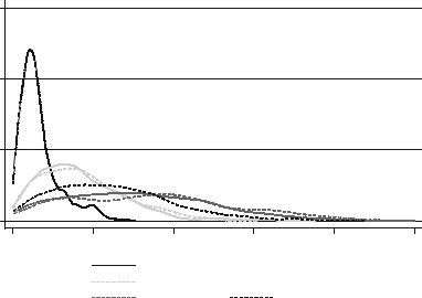
168 |
G. Marin |
1.5 |
|
|
|
|
|
1 |
|
|
|
|
|
.5 |
|
|
|
|
|
0 |
|
|
|
|
|
0 |
2 |
4 |
6 |
8 |
10 |
TFP gap |
|
VA/CO2 gap |
|
||
VA/NOx gap |
|
VA/SOx gap |
|
||
VA/NMVOC gap |
|
VA/CO gap |
Fig. 9.1 Distribution of productivity and environmental efficiency relative gaps
sectors (the first percentile of sectors in terms of manufacturing value added or employment) to avoid potentially great measurement errors in sector representing a negligible share of an economy. Measurement errors may depend on the fact that a very small sector could include secondary activities only, with little or misleading information on the true state of the technology and on emission efficiency of the sector in a specific country.
Figure 9.1 shows the distribution of percentage gaps in both TFP and environmental efficiency (value added per unit of emissions). Interestingly, environmental efficiency is much more dispersed than productivity with still great potentials for laggard countries and sectors to converge on more environmentally efficient technologies. The lack of convergence depends on the ‘external’ nature of environmental efficiency improvements as opposed to standard TFP improvements.
The gap is relatively small for CO2 and NOx emission efficiencies, while it is relevant for CO, SOx and NMVOC emission efficiencies. This may seem a quite surprising result, given that local pollutants are regulated more strictly than CO2 emissions at European level, with potential greater homogeneity. However, pollutants are generally reduced with end-of-pipe technology which represents a pure cost for polluting firms, while carbon dioxide emissions are very strongly correlated to energy use. The generally lower gap in CO2 efficiency could be the result of its strict correlation with energy use which is characterised by a substantial component of private benefit relative to pollutant emissions.

9 Closing the Gap? Dynamic Analyses of Emission Efficiency. . . |
169 |
9.4Empirical Results
For all emissions, I report results for various versions of the baseline model from the simplest version with no role for energy prices and TFP to the most complete version including energy prices and TFP (Tables 9.1, 9.2, 9.3, 9.4 and 9.5). A first remarkable result is the positive effect of emission efficiency improvements in the frontier country on domestic sectoral emission efficiency growth. This result is robust in all specifications and for all emissions, its magnitude ranging from an elasticity of 3–4% for CO2 emissions to an elasticity of 9–10% for SOx emissions. As expected, improvements in environmental efficiency at the frontier spill over to laggard countries with a beneficial effect on their emission efficiency growth. These positive spillovers may occur as a consequence of the diffusion of more environmental efficient technologies from ‘frontier’ countries and sectors to laggard countries and sectors.
Table 9.1 Estimates for CO2 emission efficiency
D ln(VA/CO2) |
(1) |
(2) |
(3) |
(4) |
(5) |
(6) |
D Frontier VA/CO2 |
0.0319* |
0.0384** |
0.0342* |
0.0407** |
0.0379** |
0.0404** |
Gap VA/CO2 (t 1) |
(0.0192) |
(0.0189) |
(0.0189) |
(0.0187) |
(0.0170) |
(0.0170) |
0.00530 |
0.0196*** |
0.00160 |
0.0152*** |
0.0130*** |
0.0184*** |
|
|
(0.00515) |
(0.00591) |
(0.00533) |
(0.00589) |
(0.00497) |
(0.00537) |
D Energy prices |
|
|
0.0522 |
0.0317 |
0.0611 |
0.0540 |
|
|
|
(0.144) |
(0.145) |
(0.132) |
(0.133) |
D Energy prices x |
|
|
0.142* |
0.152* |
0.0913 |
0.110 |
Gap VA/CO2 (t 1) |
|
|
(0.0791) |
(0.0781) |
(0.0718) |
(0.0715) |
D TFP |
|
|
|
|
0.981*** |
0.960*** |
|
|
|
|
|
(0.0396) |
(0.0399) |
D Frontier TFP |
|
|
|
|
0.0446* |
0.0519** |
Gap TFP (t 1) |
|
|
|
|
(0.0247) |
(0.0248) |
|
|
|
|
0.0431*** |
0.0704*** |
|
|
0.0240 |
0.0493** |
0.0244 |
0.0494** |
(0.00786) |
(0.0152) |
Constant |
0.0107 |
0.0314 |
||||
|
(0.0213) |
(0.0227) |
(0.0219) |
(0.0231) |
(0.0212) |
(0.0237) |
F |
3.008*** |
5.970*** |
3.229*** |
5.874*** |
28.81*** |
26.02*** |
R-squared |
0.0290 |
0.0703 |
0.0337 |
0.0751 |
0.268 |
0.288 |
Year dummies (F) |
5.182*** |
5.338*** |
6.198*** |
6.365*** |
8.716*** |
8.891*** |
Sector dummies (F) |
0.780 |
0.851 |
0.762 |
0.833 |
0.996 |
1.136 |
Country dummies |
|
12.08*** |
|
12.19*** |
|
5.214*** |
(F) |
|
|
|
|
|
|
Ramsey o.v. test |
0.662 |
3.590** |
0.831 |
4.813*** |
0.469 |
1.657 |
(F) |
|
|
|
|
|
|
N |
3,115 |
3,115 |
3,115 |
3,115 |
3,115 |
3,115 |
Standard errors in parentheses. *p < 0.1; **p < 0.05; ***p < 0.01

170 |
|
|
|
|
|
G. Marin |
Table 9.2 Estimates for NOx emission efficiency |
|
|
|
|||
|
|
|
|
|
|
|
D ln(VA/NOx) |
(1) |
(2) |
(3) |
(4) |
(5) |
(6) |
D Frontier |
0.0562*** |
0.0637*** |
0.0580*** |
0.0654*** |
0.0593*** |
0.0604*** |
VA/NOx |
(0.0202) |
(0.0203) |
(0.0198) |
(0.0200) |
(0.0186) |
(0.0187) |
Gap VA/NOx |
0.0148*** |
0.0328*** |
0.0100** |
0.0268*** |
0.0233*** |
0.0264*** |
(t 1) |
(0.00476) |
(0.00667) |
(0.00492) |
(0.00653) |
(0.00507) |
(0.00618) |
D Energy prices |
|
|
0.156 |
0.113 |
0.133 |
0.124 |
|
|
|
(0.187) |
(0.189) |
(0.180) |
(0.184) |
D Energy prices x |
|
|
0.185** |
0.202** |
0.146* |
0.169** |
Gap VA/NOx |
|
|
(0.0864) |
(0.0848) |
(0.0806) |
(0.0803) |
(t 1) |
|
|
|
|
|
|
D TFP |
|
|
|
|
1.016*** |
0.991*** |
|
|
|
|
|
(0.0438) |
(0.0436) |
D Frontier TFP |
|
|
|
|
0.0652** |
0.0665** |
Gap TFP (t 1) |
|
|
|
|
(0.0319) |
(0.0327) |
|
|
|
|
0.0522*** |
0.0657*** |
|
|
|
0.0470** |
|
0.0484* |
(0.00933) |
(0.0162) |
Constant |
0.00508 |
0.00264 |
0.0159 |
0.0342 |
||
|
(0.0216) |
(0.0232) |
(0.0232) |
(0.0247) |
(0.0229) |
(0.0260) |
F |
2.335*** |
5.782*** |
2.838*** |
5.850*** |
21.98*** |
22.65*** |
R-squared |
0.0248 |
0.0630 |
0.0326 |
0.0704 |
0.210 |
0.230 |
Year dummies |
3.670*** |
3.786*** |
5.034*** |
5.154*** |
6.507*** |
6.536*** |
(F) |
|
|
|
|
|
|
Sector dummies |
0.982 |
1.275 |
0.954 |
1.247 |
0.691 |
0.746 |
(F) |
|
|
|
|
|
|
Country dummies |
|
15.35*** |
|
15.02*** |
|
11.73*** |
(F) |
|
|
|
|
|
|
Ramsey o.v. test |
6.632*** |
3.234** |
3.986*** |
8.240*** |
0.178 |
0.227 |
(F) |
|
|
|
|
|
|
N |
3,115 |
3,115 |
3,115 |
3,115 |
3,115 |
3,115 |
Standard errors in parentheses. *p < 0.1; **p < 0.05; ***p < 0.01
The distance from the frontier country in terms of emission efficiency affects17 domestic emission efficiency growth positively and significantly for all emissions except NMVOC. This generally positive effect is a clear evidence of convergence in emission efficiency of laggard countries towards the emission efficiency frontier, with the speed of convergence being greater for countries and sectors with the biggest gap. It is evident from Figure 9.1 that there are huge potentials of convergence in emission efficiency performance. However, it is clear that to accelerate the rate of convergence, there is a need for further harmonisation of environmental policies across countries and additional effort made to promote the diffusion of efficient technologies. The negative effect of the efficiency gap for NMVOC is small in magnitude and insignificant when including either country fixed effects or
17 I refer here to the direct effect assuming no energy price change (Dener_pricesc,t 1 ¼ 0) in columns 3–6.

9 Closing the Gap? Dynamic Analyses of Emission Efficiency. . . |
|
171 |
||||
Table 9.3 Estimates for NMVOC emission efficiency |
|
|
|
|||
|
|
|
|
|
|
|
D ln(VA/ |
|
|
|
|
|
|
NMVOC) |
(1) |
(2) |
(3) |
(4) |
(5) |
(6) |
|
|
|
|
|
|
|
D Frontier |
0.0421* |
0.0484** |
0.0416* |
0.0474** |
0.0425* |
0.0468** |
VA/NMVOC |
(0.0240) |
(0.0243) |
(0.0237) |
(0.0239) |
(0.0234) |
(0.0236) |
Gap VA/NMVOC |
0.0122*** |
0.00156 |
0.00803** |
0.00424 |
0.00281 |
0.00503 |
(t 1) |
(0.00353) |
(0.00451) |
(0.00343) |
(0.00496) |
(0.00351) |
(0.00488) |
D Energy prices |
|
|
1.105** |
1.099** |
1.073** |
1.054** |
|
|
|
(0.446) |
(0.455) |
(0.441) |
(0.453) |
D Energy prices x |
|
|
0.123 |
0.115 |
0.125 |
0.113 |
Gap VA/NMVOC |
|
|
(0.0828) |
(0.0825) |
(0.0819) |
(0.0822) |
(t 1) |
|
|
|
|
|
|
D TFP |
|
|
|
|
0.939*** |
0.908*** |
|
|
|
|
|
(0.0568) |
(0.0584) |
D Frontier TFP |
|
|
|
|
0.0523 |
0.0518 |
Gap TFP (t 1) |
|
|
|
|
(0.0385) |
(0.0382) |
|
|
|
|
0.0319*** |
0.0532** |
|
|
|
0.0119 |
|
0.0452 |
(0.0109) |
(0.0210) |
Constant |
0.0549** |
0.0181 |
0.0287 |
0.0335 |
||
|
(0.0246) |
(0.0265) |
(0.0295) |
(0.0330) |
(0.0285) |
(0.0321) |
F |
3.261*** |
4.919*** |
3.196*** |
4.754*** |
14.81*** |
16.03*** |
R-squared |
0.0373 |
0.0676 |
0.0479 |
0.0777 |
0.139 |
0.159 |
Year dummies (F) |
2.119** |
2.035** |
2.967*** |
2.928*** |
3.289*** |
3.246*** |
Sector dummies |
3.155*** |
2.098*** |
3.032*** |
2.112*** |
3.462*** |
2.778*** |
(F) |
|
|
|
|
|
|
Country dummies |
|
7.374*** |
|
7.223*** |
|
6.438*** |
(F) |
|
|
|
|
|
|
Ramsey o.v. test |
15.64*** |
172.9*** |
148.9*** |
253.8*** |
35.27*** |
93.40*** |
(F) |
|
|
|
|
|
|
N |
3,115 |
3,115 |
3,115 |
3,115 |
3,115 |
3,115 |
Standard errors in parentheses. *p < 0.1; **p < 0.05, ***p < 0.01
TFP growth (domestic and frontier country) and gap. Unlike other types of emission, NMVOC emission efficiency is not characterised by convergence patterns.
The coefficient for the change in energy prices (b6) describes the effect of prices on emission efficiency growth as if the sector were the technological leader, whereas the actual effect of prices is given by b6 + b7*gap_ln(VAc,s,t 1/Ec,s,t 1). The effect on frontier sectors is always positive although it is significant for NMVOC and CO emissions only. The interaction term, on the other hand, has a positive effect for CO2, NOx and SOx (weakly significant for CO2, significant for NOx and not significant for SOx) and a negative effect for NMVOC (though not significant) and CO (significant). A positive effect means that the effect of energy price changes on emission efficiency growth is increasing in the gap in emission efficiency from the frontier country, making laggard countries more sensitive to price changes than frontier countries. When computing marginal effects, the effect of energy prices for CO2, NOx and SOx increases with distance from the frontier.

172 |
|
|
|
|
|
G. Marin |
Table 9.4 Estimates for SOx emission efficiency |
|
|
|
|||
|
|
|
|
|
|
|
D ln(VA/SOx) |
(1) |
(2) |
(3) |
(4) |
(5) |
(6) |
D Frontier VA/SOx |
0.0901*** |
0.0965*** |
0.0902*** |
0.0963*** |
0.0926*** |
0.0979*** |
Gap VA/SOx (t 1) |
(0.0229) |
(0.0232) |
(0.0228) |
(0.0231) |
(0.0229) |
(0.0230) |
0.0467*** |
0.0605*** |
0.0452*** |
0.0582*** |
0.0521*** |
0.0608*** |
|
|
(0.00740) |
(0.00882) |
(0.00785) |
(0.00912) |
(0.00894) |
(0.00935) |
D Energy prices |
|
|
0.475 |
0.380 |
0.398 |
0.282 |
|
|
|
(0.365) |
(0.362) |
(0.363) |
(0.360) |
D Energy prices x |
|
|
0.0753 |
0.0864 |
0.0684 |
0.105 |
Gap VA/SOx (t 1) |
|
|
(0.0949) |
(0.0944) |
(0.0947) |
(0.0932) |
D TFP |
|
|
|
|
0.861*** |
0.907*** |
|
|
|
|
|
(0.0917) |
(0.0969) |
D Frontier TFP |
|
|
|
|
0.000683 |
0.0368 |
Gap TFP (t 1) |
|
|
|
|
(0.0759) |
(0.0752) |
|
|
|
|
0.0697*** |
0.151*** |
|
|
|
0.00240 |
|
0.0118 |
(0.0247) |
(0.0451) |
Constant |
0.0380 |
0.0251 |
0.0552 |
0.0485 |
||
|
(0.0371) |
(0.0472) |
(0.0393) |
(0.0471) |
(0.0393) |
(0.0496) |
F |
4.888*** |
5.329*** |
4.926*** |
5.316*** |
7.387*** |
7.263 *** |
R-squared |
0.0580 |
0.0660 |
0.0610 |
0.0684 |
0.0882 |
0.0981 |
Year dummies (F) |
7.833*** |
7.928*** |
8.220*** |
8.342*** |
8.384*** |
8.028*** |
Sector dummies (F) |
2.778*** |
3.087*** |
2.758*** |
3.045*** |
3.354*** |
3.862*** |
Country dummies |
|
2.716*** |
|
2.458*** |
|
2.644*** |
(F) |
|
|
|
|
|
|
Ramsey o.v. test (F) |
47.20*** |
48.42*** |
47.88*** |
49.15*** |
11.55*** |
9.017*** |
N |
3,115 |
3,115 |
3,115 |
3,115 |
3,115 |
3,115 |
Standard errors in parentheses. *p < 0.1; **p < 0.05; ***p < 0.01
The overall effect of energy prices turns out to be positive and significant (10% already at the first quartile of emission efficiency gap). For these emissions, energy prices trigger significant improvement in laggard countries, while the emission efficiency frontier is not significantly affected. Other factors seem to drive emission efficiency improvement at the frontier, probably related to domestic technological capability and experience in environmental technologies. Preliminary results (available upon request) using the number of environmental patent applications per unit of GDP instead of energy prices indicate a positive significant direct effect (b6) on emission efficiency for CO2 and NOx.
On the contrary, the marginal effect of energy prices decreases in the emission efficiency gap for NMVOC and CO emissions even though it is still strongly significant at the 90th percentile of the emission efficiency gap. In these cases, energy price dynamics is a stronger incentive for sectors that are close to the emission efficiency frontier than for laggard sectors. A possible explanation for the opposite results relative to CO2, NOx and SOx regarding the effect of energy prices may be related to opposite patterns of environmental technological change for laggards and frontier sectors. On the one hand, laggard sectors seem to focus on the improvement of energy efficiency (strongly correlated with CO2 efficiency) and

9 Closing the Gap? Dynamic Analyses of Emission Efficiency. . . |
|
173 |
||||
Table 9.5 Estimates for CO emission efficiency |
|
|
|
|||
|
|
|
|
|
|
|
D ln(VA/CO) |
(1) |
(2) |
(3) |
(4) |
(5) |
(6) |
D Frontier VA/CO |
0.0758*** |
0.0789*** |
0.0734*** |
0.0769*** |
0.0760*** |
0.0771*** |
Gap VA/CO (t 1) |
(0.0258) |
(0.0259) |
(0.0251) |
(0.0253) |
(0.0245) |
(0.0247) |
0.0152*** |
0.0240*** |
0.0194*** |
0.0280*** |
0.0257*** |
0.0276*** |
|
|
(0.00476) |
(0.00622) |
(0.00505) |
(0.00666) |
(0.00534) |
(0.00646) |
D Energy prices |
|
|
1.438*** |
1.335*** |
1.450*** |
1.381*** |
|
|
|
(0.406) |
(0.393) |
(0.398) |
(0.392) |
D Energy prices x |
|
|
0.225** |
0.196* |
0.273** |
0.237** |
Gap VA/CO (t 1) |
|
|
(0.107) |
(0.102) |
(0.107) |
(0.102) |
D TFP |
|
|
|
|
1.042*** |
1.013*** |
|
|
|
|
|
(0.0753) |
(0.0768) |
D Frontier TFP |
|
|
|
|
0.0688 |
0.0720* |
Gap TFP (t 1) |
|
|
|
|
(0.0428) |
(0.0431) |
|
|
|
|
0.0575*** |
0.0789*** |
|
|
|
0.00121 |
0.0255 |
0.0425 |
(0.0129) |
(0.0251) |
Constant |
0.0191 |
0.00601 |
0.0236 |
|||
|
(0.0314) |
(0.0340) |
(0.0355) |
(0.0386) |
(0.0343) |
(0.0381) |
F |
2.541*** |
6.218*** |
2.626*** |
5.936*** |
10.71*** |
13.99*** |
R-squared |
0.0380 |
0.0756 |
0.0533 |
0.0883 |
0.143 |
0.168 |
Year dummies |
1.685* |
1.733* |
2.889*** |
2.832*** |
3.445*** |
3.113*** |
(F) |
|
|
|
|
|
|
Sector dummies |
2.418*** |
2.415*** |
2.419*** |
2.414*** |
2.367*** |
2.150*** |
(F) |
|
|
|
|
|
|
Country dummies |
|
16.21*** |
|
14.58*** |
|
11.39*** |
(F) |
|
|
|
|
|
|
Ramsey o.v. test |
3.265** |
96.58*** |
47.25*** |
166.7*** |
53.05*** |
116.5*** |
(F) |
|
|
|
|
|
|
N |
3,115 |
3,115 |
3,115 |
3,115 |
3,115 |
3,115 |
Standard errors in parentheses. *p < 0.1; **p < 0.05; ***p < 0.01
on the abatement of more ‘classical’ pollutants such as SOx and NOx. On the other hand, sectors lying close to the emission efficiency frontier seem to be characterised by fewer energy inefficiencies (and, consequently, higher marginal costs to improve energy efficiency) and by higher marginal costs for the abatement of classical pollutants due to the long tradition of stringent environmental standards.
The inclusion of productivity measures (total factor productivity – TFP – growth in the sector and in the frontier country and TFP gap from the frontier) in the last two columns does not affect the estimates of other parameters. However, considering TFP has the consequence of improving substantially the goodness of fit (R-squared).18 As expected, the relationship between sectoral TFP growth and emission efficiency growth is positive and strongly significant, with coefficients varying from a minimum of 0.86 (SOx without country fixed effects) to 1.04
18 No relevant improvements in the R-squared are found for SOx estimates where the gain is of about 2–3% of explained variance.
174 |
G. Marin |
(CO without country fixed effects). This means that an increase in TFP translates into a very similar increase in emission efficiency conditional on other covariates. This very robust result highlights the strong complementarity between economic productivity and environmental efficiency. The effect of TFP growth in the frontier country has a generally negative effect on emission efficiency growth, with the coefficient being statistically significant just for CO2 (5%), NOx (5%) and CO (10% only when including country fixed effects, insignificant otherwise). The insignificant or negative effect of TFP growth in the frontier country may suggest that frontier technological change is not explicitly directed to improve emission efficiency and, in some cases, there is a weak evidence of ‘emission-intensive’ technical change. Finally, the gap in TFP from the frontier country negatively and significantly affects emission efficiency growth in all cases. The existence of a negative effect of TFP gap further stresses the complementarity links between economic and environmental performance, especially since differences in emission efficiency were already accounted for. As stated in the previous section, results employing alternative measures of TFP or using labour productivity give rise to qualitatively very similar estimates.
Some considerations on year, sector and country fixed effects are needed. Year and country dummies are jointly strongly significant in all specifications and for all emissions. Significant Europe-wide time dummies possibly highlight the relevance of regulatory efforts at the European level affecting all countries.
Sector dummies, on the contrary, are not jointly significant for both CO2 and NOx estimates, highlighting quite uniform efficiency patterns among sectors within countries for these types of emissions. On the contrary, they are jointly strongly significant for SOx, NMVOC and CO, highlighting heterogeneous patterns of emission efficiency potentially driven by sector-specific environmental regulations.
Country dummies are jointly strongly significant in all cases, stressing the great heterogeneity of environmental efficiency and highlighting the relevance of systematic differences among countries in emission efficiency dynamics even after controlling for the gap in environmental efficiency and productivity.
Results reported in this chapter do not change substantially when performing some simple robustness checks. The inclusion of outliers or small sectors does not influence either the magnitude or the significance of estimated coefficients. The use of more aggregate sector information, for example, at the level of subsection NACE with 14 manufacturing sectors, reduces the significance of many coefficients, but the magnitude does not change. When removing specific countries or sectors (one by one) the magnitude of estimated coefficients does not change substantially even if significance is generally lower. Finally, tests on the presence of structural breaks in estimated coefficients were performed.19 No significant structural break was
19 I performed a Chow test by interacting a dummy variable identifying a specific time period with all covariates in the model described by Eq. 9.2. The test (a simple F-test) is performed by assuming, under the null hypothesis, that the parameters of all interaction terms are jointly equal to zero, thus indicating no structural break.

9 Closing the Gap? Dynamic Analyses of Emission Efficiency. . . |
175 |
found for CO2 and NMVOC emissions. Statistically significant breaks were found for NOx (1998 and 2000), SOx (2005) and CO (1999, 2001, 2002 and 2005) even though just three of them were significant at the 1% level (NOx 2000, SOx 2005 and CO 1999).
9.5Conclusions
This chapter investigates the dynamics of sectoral emission efficiency in a selection of European countries. International diffusion of more efficient environmental technologies, distance from the technological frontier, energy prices and economic productivity patterns are found to be important drivers of emission efficiency growth in manufacturing sectors.
Results highlight the importance of the diffusion of more environmentally efficient production technologies from leader countries to laggards. However, the channels through which the diffusion occurs are not investigated directly. The convergence of emission efficiency towards the frontier is faster for countries and sectors with a greater efficiency gap, probably showing evidence of increasing marginal costs of abatement. Energy price dynamics has a positive effect on emission efficiency, and the effect is decreasing in the emission efficiency gap for CO and NMVOC emission efficiency growth, while it is significant only for laggard sectors (and increasing in the emission efficiency gap) for CO2, NOx and SOx emission efficiency growth. Moreover, there is a very robust evidence of complementarity between emission efficiency and economic productivity (here measured with TFP). Finally, the homogeneity of estimates across different types of air emissions is quite surprising, especially in the presence of moderate pairwise correlation between emission efficiency growth rates.20
Based on the evidence discussed in this chapter concerning the international diffusion of emission efficiency, further research is needed to investigate the way through which sectors in laggard countries take advantage of emission efficiency improvements occurring in the frontier countries. As discussed in the introduction, the diffusion of environmental technologies leading to improvement in emission efficiency may be triggered by a variety of factors. The assessment of the contribution to the diffusion of environmental technologies of these factors is crucial to identifying the optimal policy mix. Finally, it is worth combining patterns of international diffusion with patterns of cross-sectoral diffusion within the same country (Corradini et al. 2011) in a comprehensive framework to obtain a more complete representation of the diffusion of emission efficient technologies.
20 Pairwise correlation between emission efficiency growth rates is greater than 50% in just three cases (CO2-NOx, 70%; CO-NMVOC, 60.21%; NOx-CO, 60.16%) and is lower than 20% in one case (19.59% for NMVOC-SOx).
176 |
G. Marin |
Appendix: Air Emission Features
Emissions differ substantially as regards the ‘external cost’ they produce. Carbon dioxide emissions have no direct effect on health and on local communities, whereas they contribute to the greenhouse effect and global climate change. On the contrary, other emissions (NOx, SOx, NMVOC and CO) have serious effects on health and damage the environment at the local level through acidification (NOx and SOx), ozone depletion (NOx), eutrophication (NOx) and tropospheric ozone formation (CO and NOx).
These differences resulted in different timing and characteristics of national or supranational regulations. Pollutant emissions have been regulated at the European level since the mid-1980s through a series of directives which have eased the harmonisation of national policies. Among others, the following directives aimed at regulating pollution should be taken into account. The Sulphur Dioxide Air Pollution Directive, approved in 1980 (1980/779/EEC), aimed at reducing SOx emissions, while the Nitrogen Dioxide Air Pollution Directive approved in 1985 (1985/203/EEC) focused on the reduction of NOx emissions. They were replaced by the First Daughter Directive ‘Sulphur Dioxide, Nitrogen Dioxide and Oxides of Nitrogen, Particulate Matter and Lead in Ambient Air’ in 1999 (99/30/EC) broadening the scope of pollutant reductions to SOx and other local pollutants. The Fuel Quality Directive introduced in 1998 (98/70/EC), revised in 2003 (2003/17/EC) and in 2009 (2009/30/EC), sets specific requirements for the quality of fuels in order to reduce emissions of pollutant substances. The NEC (National Emission Ceilings) Directive (2001/81/EC), approved by the European Commission in 2001, sets legally binding limits to national emissions of NOx, SO2, NMVOC and ammonia. Finally, a broader programme to consider air pollution emissions in a comprehensive way was launched by the European Commission in 2005 (Clean Air for Europe programme – CAFE).
On the contrary, regulatory efforts explicitly aimed at reducing carbon dioxide emissions were less effective. No relevant policy was introduced before the approval of the Kyoto Protocol (1997), and, even after the protocol started being legally binding (2001), no real action was taken before the introduction of the emission trading scheme (in its pilot phase) in 2005 and the ‘20-20-20’ strategy proposed in 2007.
References
Carrio´n-Flores, C. E., & Innes, R. (2010). Environmental innovation and environmental performance. Journal of Environmental Economics and Management, 59, 27–42.
Cole, M. A., Elliott, R. J. R., & Shimamoto, K. (2005). Industrial characteristics, environmental regulations and air pollution: An analysis of the UK manufacturing sector. Journal of Environmental Economics and Management, 50, 121–143.
9 Closing the Gap? Dynamic Analyses of Emission Efficiency. . . |
177 |
Corradini, M., Costantini, V., Mancinelli, S., & Mazzanti, M. (2011). Environmental and innovation performance in a dynamic impure public good framework (Departmental Working Papers of Economics, No. 0141). Universita` ‘Roma Tre’.
Costantini, V., & Mazzanti, M. (2012). On the green side of trade competitiveness? The impact of environmental policies and innovation on EU exports. Research Policy, 41(1), 132–153.
Jaffe, A., Newell, R. G., & Stavins, R. N. (2005). A tale of two market failures: Technology and environmental policy. Ecological Economics, 50(2–3), 164–174.
Lanjouw, J. O., & Mody, A. (1996). Innovation and the international diffusion of environmentally responsive technology. Research Policy, 25, 549–571.
Lovely, M. & Popp, D. (2011). Trade, technology, and the environment: Does access to technology promote environmental regulation? Journal of Environmental Economics and Management, 61(1), 16–35.
Marin, G., & Mazzanti, M. (2010). The evolution of environmental and labour productivity dynamics – Sector analyses and decoupling/recoupling trends on a 1990–2007 Italian NAMEA. Journal of Evolutionary Economics.
Mazzanti, M., & Musolesi, A. (2010). Carbon abatement leaders and laggards – Non parametric analyses of policy oriented Kuznets curves. Nota di Lavoro FEEM 149.2010. Fondazione Eni Enrico Mattei, Milan.
Mazzanti, M., & Zoboli, R. (2009). Environmental efficiency and labour productivity: Trade-off or joint dynamics? A theoretical investigation and empirical evidence from Italy using NAMEA.
Ecological Economics, 68(4), 1182–1194.
Moomaw, W. R., & Unruh, G. C. (1997). Are environmental Kuznets curves misleading us? The case of CO2 emissions. Environment and Development Economics, 2, 451–463.
Newell, R. G., Jaffe, A. B., & Stavins, R. N. (1999). The induced innovation hypothesis and energy-saving technological change. Quarterly Journal of Economics, 114(3), 941–975.
Nicoletti, G., & Scarpetta, S. (2003). Regulation, productivity and growth: OECD evidence.
Economic Policy, 18(36), 9–72.
Popp, D. (2002). Induced innovation and energy prices. The American Economic Review, 92(1), 160–180.
Popp, D. (2006). International innovation and diffusion of air pollution control technologies: The effects of NOx and SO2 regulation in the US, Japan and Germany. Journal of Environmental Economics and Management, 51, 46–71.
Popp, D., Newell, R. G., & Jaffe, A. B. (2009). Energy, the environment and technological change
(NBER Working Papers 14832). National Bureau of Economic Research, Inc.
Porter, M. E., & Van Der Linde, C. (1995). Toward a new conception of the environmentcompetitiveness relationship. Journal of Economic Perspectives, 9(4), 97–118.
Scarpetta, S., & Tressel, T. (2002). Productivity and convergence in a panel of OECD industries: do regulations and institutions matter? (OECD Economics Department Working Papers No. 342). Paris: OECD Publishing. doi: 10.1787.004581482564.

Chapter 10
Waste Technological Dynamics and Policy Effects: Evidence from OECD Patent Data
Francesco Nicolli
Abstract This chapter examines the effect of environmental policies on technological change, in the field of waste management. This study is conducted using patent data on 28 OECD countries over the period 1980–2005 and considers five different technological fields related to the waste sector. Even though the analysis confirms that policies actually played a positive, significant role in promoting the development of green innovations, this effect is highly non-linear and strongly depends on time. As previous works have highlighted, the technological maturity of the sector, especially if compared with other areas of environmental innovation such as renewables, is reflected in a decreasing effect of policies on innovation trends. If a first wave of policies, which dates back to the 1990s, was able to promote technological change, this effect is now less evident. Nevertheless, it is reasonable to conclude that if no policy efforts had been introduced, the slowdown in the trend of patenting in waste-related sectors would have been even more pronounced.
Keywords Waste management • Patents • Policy effects • Non linearity • Technology fields
10.1Introduction
Landfill reduction has been, in the last decades, one of the primary aims of environmental policies in European and OECD countries. According to the European waste hierarchy, landfill diversion and waste prevention are the two main priorities in the new waste management strategies. For this reason, in 1999,
F. Nicolli (*)
Department of Economics & Management, University of Ferrara,
Via Voltapaletto 11, Ferrara, Italy
CERIS CNR Milan, Via Bassini 15, Milan e-mail: francesco.nicolli@unife.it
V. Costantini and M. Mazzanti (eds.), The Dynamics of Environmental |
179 |
and Economic Systems: Innovation, Environmental Policy and Competitiveness,
DOI 10.1007/978-94-007-5089-0_10, # Springer Science+Business Media Dordrecht 2013
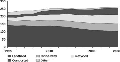
180 |
F. Nicolli |
Fig. 10.1 Development of municipal waste management in EU-27 (Millon ton)
a European landfill directive was issued (EEA 2007), which can still be considered the cornerstone of European waste strategy. This policy measure, like many other European guidelines on waste, has to be accepted and implemented at country level because the goals set by the directive can only be achieved by a decentralised implementation associated with further national legislation.
Despite all the efforts, landfilling is still a very important option in the European municipal waste management but with significant differences among the European countries. The two pictures below, for example, tell us two different and important stories. Figure 10.1 shows how, at an aggregate level, the composition of waste management has changed radically from 1995 to 2008, with a declining trend in landfilling in favour of more preferred disposal options such as recycling, incineration and composting. If the general picture looks extremely positive, the second graph below (Fig. 10.2) shows how the aggregate data masks high intra-country heterogeneity. For example, there are countries, such as Germany, Sweden and Belgium, that rely on landfilling only for a very small share of the total waste management (less than 5%), and there is a second group of countries, including Italy, Finland and Spain, in which landfilling accounts for about the 50% of the total waste management. Finally, there is a last group that includes, among others, Lithuania, Greece and Bulgaria, in which landfill is still the predominant disposal choice.
Furthermore, even if the pictures above depict a positive trend of general waste management in Europe, the total amount of waste produced is continuously increasing (EEA 2010) in EU-27, driven mainly by household consumption and the increasing number of households. This increasing amount of waste production puts pressure on the management system, with a consequent increase in the amount of waste traded across borders, much of it for recycling and energy recovery.
In this context, policy stringency may play many important roles. First of all, policy may be implemented at country level in order to promote landfill diversion and to encourage the use of other forms of disposal, such as recycling and incineration. For these cases, a mix of command-and-control and economic instruments is

10 Waste Technological Dynamics and Policy Effects. . . |
181 |
Fig. 10.2 Municipal waste landfilled in EEA countries (share of total disposal)
generally implemented. These are bans on landfilling of specific materials, technical requirements for the construction of landfill sites and incineration plants, landfill tax and specific limits on the heavy metal contained in packaging, etc. Moreover, many countries have adopted a polluter pays principle scheme (i.e., they have shifted the responsibility from the consumer to the producer) as in plastic and paper packaging. European directives, on the other hand, generally impose specific performance targets (such as a share of waste to be recycled), with flexibility in the adoption of the preferred technology. In addition to the emphasis posed by the European waste hierarchy, the focus on landfill reduction is due in part to the negative environmental impacts of landfilling (Pearce 2004) that, in many cases, are not economically justified, especially if the cost and benefit of different waste management technologies are taken into account (Dijkgraaf and Vollebergh 2004). Secondly, in a context that is evolving rapidly and in which the main technological paradigm (disposal) is switching to new and differentiated alternatives, it is interesting to understand what role policy stringency has played in promoting technical change (Johnstone et al. 2010b). The first of these two points has been the object of a consolidated strand of literature, while the second point, the relationship between policy stringency and environmental innovation, is the aim of this work. Thanks to an online database made available by the OECD,1 we can study how waste-related technologies have changed among a selected group of 28 OECD countries in the period 1980–2005, through the analysis of patent data. In particular, the OECD online statistic service divides waste-related patents into five classes: incineration and recovery, material recycling, fertilisers from waste, solid waste collection and
1 OECDStatExtract, available at http://stats.oecd.org

182 |
F. Nicolli |
general waste management. Starting from this data, five innovation indicators have been created at country level for the analysed period, and they will be used in the following section as proxies for environmental innovation at country level. Moreover, a series of country fact sheets on environmental regulation, made available by Eionet,2 have made it possible to create a policy indicator that will be used to test the effect of regulation on environmental innovation. This chapter is structured as follows: the first section illustrates the main characteristics of the two strands of relevant literature, that is, waste management and disposal options, and the drivers of environmental innovation; the second section illustrates the data and the methodology used in the analysis; the third one presents the main results of an econometric analysis conducted on the data and their economic interpretation; and the final section concludes.
10.2Waste, Environmental Policies and Technological Innovation
An important part of the waste literature is related to waste management and the evaluation of the externalities involved with the different instruments of waste recovery, with many focusing on cost-benefit analyses of different waste management strategies, often accompanied by policy indications and evaluations. A good survey of this branch of literature can be found in Goddard (1995) and Choe and Fraser (1998). In addition to these studies on waste management, another much smaller (in terms of number of publications) body of literature has been built up in the last decade with the aim to understand the evolution of waste generation and disposal over time. Even though these kinds of studies are not directly correlated with this analysis, this work strongly refers to this branch of literature for the identification of the possible determinant of waste management development. These studies, based on Kuznets-type models, aim at understanding how waste generation and waste disposal evolve when income rises, usually by regressing the environmental (waste) indicator variable against GDP and squared GDP, with the purpose of testing for the presence of delinking between environmental impact and economic growth. A common result of this literature is that there is still no evidence of an inverted U-shape in relation to waste generation (the amount of waste generated is increasing with respect to income) but a general change in the composition of waste management is usually registered. What usually happens, in fact, is that, with respect to GDP, landfilling generally decreases (i.e., we have absolute delinking) or increases less than proportionally (the so-called relative delinking) with respect to income, whereas incinerating and recycling usually increase with respect to income. Cole et al. (1997) was one of the first studies of this kind, and the
2 EIONET is a partnership agency of the EEA and its member countries; it is fundamental to the collection and organisation of data for the EEA. See www.eionet.net
10 Waste Technological Dynamics and Policy Effects. . . |
183 |
authors found a monotonically increasing relationship between income growth and waste accumulation in relation to municipal solid waste using a data set of 13 OECD countries over 15 years (1975–1990); Seppala et al. (2001) in a study on industrialised country over the period 1970–1994 found the same result. Regarding waste disposal, Fischer-Kowalski and Amann (2001) found evidence of absolute delinking for landfilled waste but only a relative delinking for generated waste by analysing OECD countries over the period 1975–1995. Kaurosakis (2006) obtained similar results by conducting a similar analysis on 30 OECD countries including some socio-economical and policy-oriented variables. Finally, Mazzanti and Zoboli (2005) found no evidence of either absolute or negative delinking in Europe during the period 1995–2000. More recently, Mazzanti et al. (2009a) in an analysis at EU level confirmed that municipal solid waste is constantly increasing with respect to income, while a more reassuring picture is emerging from landfilling and recycling. Environmental policy in the field of waste is in fact driving a transaction towards a progressive reduction in landfilling and a consequent promotion of recycling and incineration, even if disparities are still present among countries. Finally, in an analysis of the Italian case conducted at provincial level, Mazzanti et al. (2012) found that here too, we are in the presence of absolute decoupling for landfilled waste, but the total amount of waste is still increasing with income. Summarising the results of this first strand of literature, the waste management in OECD countries is characterised by a flow of total generated waste that is monotonically increasing with respect to income, whereas landfilling is, on average, decreasing and incineration and recycling are increasingly becoming more important. As the above-mentioned literature tells us, this transaction has been partially driven by policy stringency, as well as other socio-economic factors. Nevertheless, these results leave an open question. The policy adopted in OECD countries may have had an effect on the innovative performances of the waste management sector, generating an incentive for a continuous search for more economically efficient ways of meeting the new target posed by the regulation. Debates of this kind are not new in environmental economics, even though they have rarely been applied to waste management studies. Up to 20 years ago, the economic discipline was dominated by the idea that since firms are profit maximising, any attempt by environmental regulation to abate pollution would lead to an increase in internal costs for the compliant firm. In this framework of analysis in fact, if profitable opportunities existed to reduce pollution, optimising firms would certainly already have taken advantage of them. Moreover, many theoretical studies during the 1970s give support to the idea that a country comparative advantage could have been affected in a negative manner by stringent environmental regulation. For instance, the works of Pethig (1975), Siebert (1977) and McGuire (1982) stress how environmental policies increasing firms’ internal costs affect countries competitiveness by decreasing exports, increasing imports and lowering the general country’s capacity to compete in an international market. Moreover, in the long run, if production factors are free to move across countries, more stringent environmental regulation can produce movement of the manufacturing capacity from more regulated countries to less regulated ones (which are often called “pollution havens” in modern
184 |
F. Nicolli |
environmental and trade studies). From this perspective, command-and-control regulation, for example, that restricts the choice of technologies or inputs in the production process would increase the constraints a firm has to face, while taxes and tradable permits, charging production by-products (wastes or emissions), generate costs that did not exist before the regulation. Nevertheless, in the last two decades, many scholars have challenged this main idea. In different contributions, Porter and van der Linde (1991, 1995) strongly criticised this approach, underlining that the consolidated paradigm did not consider all the aspects of the environmental regulation/competitiveness relationship. Moving from the static approach in which technology was held constant to a dynamic context, the authors showed how in practice some of the loss of competitiveness related to the environmental regulation was compensated for by an increase in innovation driven by the policy itself. According to Porter and van der Linde in fact, a proper design policy framework may put pressure on firms, pushing them to develop new innovations and promoting technological change. From this point of view, this additional policy-driven innovation may offset the loss of competitiveness due to the additional costs of regulation. In particular, Porter and van der Linde show how regulation can act through six different channels (1995). First, regulation signals likely resource inefficiencies and potential technological improvements to companies; second, regulation focused on information gathering can achieve major benefits by raising corporate awareness; third, regulation reduces the uncertainty in environmental pollution activities; fourth, regulation, posing pressure on firm cost function, motivates cost-saving innovations; and fifth, regulation makes free riding behaviour in the transition phase through an innovation-based equilibrium more difficult. Based on this seminal work, Jaffe and Palmer (1995) distinguished three different implications of the Porter hypothesis, proposing a taxonomy, that is helpful in discerning the different lines of research that have further developed. The first idea, also called narrow Porter hypothesis, shows that certain types of environmental regulations are able to stimulate innovation, based on the idea that policy design matters and command-and-control policies are generally (with exceptions) less efficient than economic instruments in promoting innovation and technical change. A second version of the Porter hypothesis, called weak, states in a nutshell that a well-designed environmental regulatory system may stimulate certain kinds of innovation. Finally, the stronger version of the Porter hypothesis says that regulation is not only able to spur innovation but also that this gain in efficiency is able to completely offset the loss in competitiveness due to compliance costs. In other terms, this last approach suggests that more stringent and well-designed regulation promotes competitiveness.
Porter’s original idea has been strongly criticised, especially by Oates et al. (1995) and Palmer et al. (1997). These authors suggest that the entire Porter reasoning was based on wrong assumptions that were not compatible with the concept of profit-maximising firms. Nevertheless, this is the exact point stressed by Porter himself. In his view, firms operate in a dynamic and uncertain framework, where the agent behaves according to Simon’s idea of bounded rationality. In such a context, the rationality of firms is moved by managers who may have different
10 Waste Technological Dynamics and Policy Effects. . . |
185 |
objectives from the firm or do not have the competence to innovate at an adequate level. Following this line of reasoning, some theoretical works explained the Porter hypothesis as being due to managers who are risk adverse (Kennedy 1994), resistant to costly changes in their routines (Ambec and Barla 2007) or rationally bounded (Gabel and Sinclair-Desgagne´ 1998). Ambec and Barla (2002), on the other hand, argue that whenever managers have private information on the outcome of R&D investments and the government does not, a problem of asymmetric information may rise from which managers may derive a rent. On the contrary, if a government enacts stringent environmental regulation, it can deprive managers of their advantage and overcome this problem. Obviously, the presence of this inefficiency supports the presence of the Porter hypothesis.
In addition to the discussed theoretical contributions, the core debate regarding the Porter hypothesis has been developed through a number of different empirical studies. Following the survey conducted by Ambec et al. (2010),3 these works can be divided into three different macro sections, representing the three different connotations of the PH, respectively: weak, strong and narrow.
With regard to the first group of works, referring conceptually (and often not explicitly) to the so-called “weak” version, one of the first contributions is Jaffe and Palmer (1997), which tested for the presence of a Porter hypothesis using pollution abatement expenditure as a proxy for environmental regulation, and total firm R&D expenditure and the total number of patent applications in a panel of US manufacturing industries in the period 1973–1991 as a proxy for innovation. Their findings support the idea that compliance expenditure has a positive and significant effect on innovation measured as R&D whereas they did not find significant results in the patent-related specifications. This last unexpected result may be due to the nature of the dependent variable: the authors used total patent counts, instead of using environmentally related ones. In another work in the same line, Brunnermeier and Cohen (2003) used US manufacturing industry data and empirically analysed the determinants of environmental technological innovation, using the number of environmental patent applications as an innovation proxy, and both pollution abatement expenditures and the number of air and water pollution control inspections as regulation proxies. They found a significant impact of the first variable and a not significant impact of the second one. Among other covariates, they found that international competition stimulates environmental innovation. Another work on patent data at firm level is Popp (2003), which by analysing 186 plants in the USA from 1972 to 1997 found that the tradable permit scheme for the reduction of SO2 has been able to promote technical change, increasing SO2 removal efficiency and decreasing operating and removal costs. Moving to cross-country studies, De Vries and Withagen (2005) studied the effect of SO2 environmental regulation on national patent counts in relative technological classes and found some evidence of a link between policy stringency
3 Ambec, S., Cohen, M. K., Elgie, S., Lanoie, P., (2011). The Porter Hypothesis at 20: Can Environmental Regulation Enhance Innovation and Competitiveness. Paper presented at Montreal, 2010 EAERE conference
186 |
F. Nicolli |
and environmental innovation. More recently, a second example of a cross-country study is Johnstone et al. (2010a), who studied the effect of many different policy instruments on the innovative performance of the main renewable technologies (solar, wind, geothermal, ocean, biomass and waste), for 15 OECD countries, over the period 1978–2003. They found strong evidence of a Porter hypothesis. In most of their specifications, different policy instruments are positively and significantly related to technological change, and more interestingly, they observed the effect of different policy designs on different technologies. Subsidies and feed-in tariffs are, for example, more suitable for inducing innovation on more costly technologies such as solar power, while tradable certificates show a stronger effect on technologies that closely compete with fossil fuel, such as wind power. Finally, Nicolli and Mazzanti (2011) studied the effect of environmental policies on innovation in the specific waste streams of paper and plastic packaging waste, end- of-life vehicles, composting and aggregate waste for OECD countries from 1970 to 2007. They found two important results on which this work is based: first, in specific waste streams, regulation does seem to play an important role in the promotion and diffusion of innovation, and second, they outlined how the waste sector seems to have reached a degree of technological maturity and is now experiencing a decreasing trend in patenting activities. These results seem to suggest that there have been two different policy eras in waste in OECD countries, a first and older wave of policies (end of the 1980s, beginning of the 1990s) that produced a technological shock in the system and a second and more recent wave of policy which seems to have had less impact on environmental innovation. Summarising the previous works, the literature tells us that there is a positive but variable link between stringent environmental regulation and innovation.
The second strand of literature refers to the “strong” version of the Porter hypothesis, that is, testing to see if there is a link between environmental regulation and competitiveness of the firms. A review of this literature can be found in Jaffe et al. (1995), where most of the papers reported there found a negative impact of environmental regulation on productivity. Nevertheless, more recent works by Berman and Bui (2001) and Alpay et al. (2002) found respectively that refineries in the Los Angeles area and Mexican food-processing industries experience an increase in competitiveness associated with increased regulation stringency. Moreover, Lanoie et al. (2008), in a study on 17 Quebec manufacturing sectors, have found a modest but significant effect of regulation on competitiveness once the dynamics of the process are taken into account. The original critique moved by Porter and van der Linde was in fact motivated by a lack of dynamics that affected these studies at that time. Lanoie et al. (2008) show that this lack of dynamics is still present in empirical studies, especially when competitiveness at time 0 is regressed against environmental regulation at the same point in time. This may have produced biased results because the effect predicted by Porter, if present, might have taken time to develop. For this reason, in their study, they introduce a lag of 3 or 4 years between regulation and productivity, showing how regulation reduces productivity after 1 year. However, this effect is reversed after only 2 years and becomes increasingly more evident as the lag increases. Finally, Costantini and Mazzanti (2012) test the effect of environmental regulation on export competitiveness of the
10 Waste Technological Dynamics and Policy Effects. . . |
187 |
manufacturing sector, using a gravity model for the EU15 group over the period 1996–2007. They find that generally policies do not seem to be harmful to export competitiveness, and specifically, some energy tax policies positively influence trade patterns.
Finally, a third approach is based on the narrow version of the Porter hypothesis, that is, flexible regulatory policies are more likely to promote innovation than more prescriptive forms of regulation. This approach follows Porter’s idea that the design of the policy actually matters and discerns the effect of command-and-control regulation (CAC) and economic instruments. In particular, Porter and van der Linde (1995) argue that CAC in particular have to respect three principles in order to be able to spur innovation:
1.They must leave the approach to innovation to firms and not to the regulating agency.
2.The stringency of CAC instruments must improve continuously and avoid locking in any particular technology.
3.The regulatory process must be certain and time consistent. Any uncertainty of the policy lever would increase the risk that investors face in the market, slowing down innovation.
On the other hand, market based and flexible instruments, such as emission taxes and tradable certificates, are more favourable since they leave firms freer to find the best technological solution to minimise compliance costs. A summary of this strand of literature would be beyond the scope of this work—a good review can be found in Driesen (2005), who concludes that environmental taxes provide a stronger incentive for innovation than other policy types.
10.3Research Hypothesis, Data and Methodology
As mentioned earlier, Nicolli and Mazzanti (2011) found evidence of a close relationship between innovation and environmental policies in the field of waste, especially in composting, end-of-life vehicles and plastic and paper packaging. This work was a first attempt to address the relationship between regulation and innovation in the field of waste through narrative examples and opened discussion for a more general analysis. In particular, in the present study, an empirical analysis through the use of econometric estimation is conducted with the aim of estimating the effect of policies and other factors on innovation. The main relationship that we want to test is the following one:
ðpatentitÞ ¼ ait þ b1 ðpolicyitÞ þ b2 ðtotpatentitÞ þ b3 ðGDPÞ þ eit |
(10.1) |
where i ¼ 1,. . ., 28 indexes the cross-sectional unit (country), t ¼ 1980,. . ., 2005 indexes time and ait is a constant term that controls for country fixed effect and for time effect. The dependent variable, patent counts, is measured as the total number

188 |
F. Nicolli |
of patent applications in each of the five areas of waste technologies (incineration and recovery, material recycling, fertilisers from waste, solid waste collection, general waste management). The explanatory variables include the policy variable (b1), the total number of patents per year per country (b2), and the last term is the country GDP (b1). eit captures all the residual variation. Following previous works in this field (for instance, Johnstone et al. (2010a)), we used negative binomial and Poisson models4 to estimate this relationship, given the count nature of the dependent variable (see also Maddala 1983; Cameron and Trivedi 1998). In particular, in this work, an event count is the number of patent applications, and we suppose here that the number of patents (PATENTSi,t) follows a negative binomial distribution.
10.3.1 Patent Data
It is well known in the economics debate that a good indicator of a country’s innovative output is hard to find. For this reason, researchers have used many different imperfect proxies in previous works such as research and development expenditure (Jaffe et al. 2007), the number of scientific workers and patent counts (Johnstone et al. 2010a). Of these measures, patent applications are particularly appealing to researchers for many reasons. First of all, patent counts display overall good availability both in terms of time and country coverage, and secondly, they can be easily and efficiently divided into technological fields. Each single patent in fact is classified through an International Patent Classification (IPC) code, developed at the World Intellectual Property Organisation. This tree-like classification allows technological fields to be created with different levels of detail in a way that is similar to NACE classification. For example, Section “D” contains all patents related to “textiles and papers”, while the subcategory “D 21” refers more specifically to “papermaking and production of cellulose”, “D 21 F” refers to “papermaking machines and methods of producing paper thereon” and, at the maximum level of detail, “D 21 F 11/06” refers to the hyper-specific field of patents related to “processes for making continuous lengths of paper, or of cardboard, or of wet web for fibreboard production, on papermaking machines of the cylinder type”. This coding allows very specific technological subcategories to be created that can identify specific fields of interest. For all these reasons, patent data have been long considered a useful proxy of innovation for economic research (Griliches 1990). Moreover, as Dernis and Kahn (2004) suggest, generally all economically relevant innovations are patented, and for this reason, patents can be used as a valuable proxy for a country or firm level of innovation. Nevertheless, patents also suffer some well-known criticalities. First of all, it is difficult to discern the value of
4 In the text, only negative binomial results are reported, but Poisson estimations generally confirm the presented results.
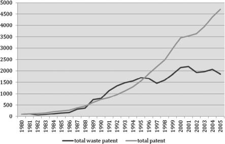
10 Waste Technological Dynamics and Policy Effects. . . |
189 |
Fig. 10.3 Number of patent application filed under the PCT (total patent and waste, 3-year moving average)
different patents. An indicator created as the sum of patent counts per year per country certainly includes patents with a high commercial and/or technological impact and patents with a lower value. Second, patent regimes and patent attitudes across country may be different. This may be due in part to legislative differences between countries and in part to a different general propensity towards patenting (in some countries, firms might be more likely to patent new inventions than in others for several different reasons. For example, in the presence of a monopoly, firms might not need a patent system to protect innovation).
For this specific analysis, we used the total amount of patents in the waste sector, divided in five different technologies, as a dependent variable. The study was carried out using patents filed under the Patent Cooperation Treaty (PCT), according to the applicant’s country of residence (and not the inventor’s country of residence). As a robustness check, we also conducted the same analysis using only patent data filed at the EPO, and the results did not change. The work was conducted on a group of 28 OECD countries, many of them European, from 1980 to 2005. The countries were Australia, Austria, Belgium, Canada, Czech Republic, Denmark, Finland, France, Germany, Greece, Hungary, Ireland, Italy, Japan, Luxembourg, Mexico, the Netherlands, New Zealand, Norway, Poland, Portugal, Slovakia, Spain, Sweden, Switzerland, Turkey, the United Kingdom and the United States. All data are taken from the OECD online patent statistics, and their trend is summarised in the two pictures below.
Figure 10.3 underlines the different development paths that total patents and waste patents exhibited from 1980 to 2005. If, on the one hand, the total patent
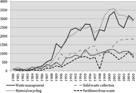
190 |
F. Nicolli |
Fig. 10.4 Number of patent application filed under the PCT (specific waste technologies, 3-year moving average)
count constantly increases through time, on the other hand, waste-related patents increased at the same pace until 1995 and then slowed down considerably. A waste technology seems more stable and less dynamic than the general trend of innovation, as already found by Nicolli and Mazzanti (2011). If we decompose the total waste patents in the five different groups (following the division made by the OECD online statistics), we can gain more insight into this trend (Fig. 10.4). Although the total amount of patents in waste-related technologies is stable, differences can be found among the different groups, with material recycling and waste management being more dynamic than the other three categories.
Figure 10.5 compares total patent applications in a selection of OECD countries that have demonstrated significant levels of waste-related innovation. The United States, Japan and Germany in particular are the three countries that present the highest number of patents, both generally and in relation to waste. Nevertheless, their trends are different. Germany and the United States show a trend for waste patents that, although different in intensity, is similar to the general one (increase until mid-1990s and than stabilisation) whereas Japan shows a completely different path of development, increasing slowly until 1999 and then registering a jump in the total number of patents filed in the field of waste.
Finally, in Fig. 10.6, we simply normalise total waste patent counts by the national GDP to obtain a measure of patent intensity that is not biased by differences in income. This procedure does not alter the ranking presented much, except for the interesting case of Italy which achieves a high level of innovation per unit of input, but is only tenth in the previous ranking based on patent counts.
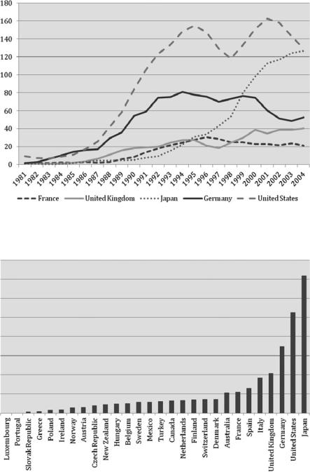
10 Waste Technological Dynamics and Policy Effects. . . |
191 |
Fig. 10.5 Number of patent application filed under the PCT (total waste patents for selected countries, 3-year moving average)
Fig. 10.6 Number of patent application filed under the PCT (total waste patent, normalised by GDP, year 2005, 3-year moving average)

192 |
F. Nicolli |
10.3.2 Relevant Policies
In order to assess the role of policy stringency on innovation, a policy indicator is constructed in this chapter based on country fact sheets on waste management available at EIONET,5 plus some additional information made available on the Ministry of Environment websites (especially for non-EU countries). Starting from this information, we constructed a series of binary variables for the different policy types in the different fields of waste. The variables take on a value of 0 prior to introduction of the policy and 1 thereafter. The variable constructed reflects the following policies:
1.Special waste: the first variable refers to the introduction, at country level, of prominent legislation in the field of special waste such as electrical waste, photographic material and pharmaceutical waste. An example of such legislation is the introduction of the EU Directive 91/157, which aimed, on the one hand, to reduce the heavy metal content of batteries and accumulators and on the other, to increase the separate disposal of spent batteries. Another example is the Directive 2002/95/EC, which supported the creation of collection schemes where consumers could return their used electronic waste free of charge. The aim of these schemes was to increase recycling and/or reuse. Moreover, this directive intended to promote the use of safe components in electrical products in order to reduce the negative externalities associated with the disposal of electrical material (it refers in particular to substituting lead, mercury, cadmium and hexavalent chromium and flame retardants such as polybrominated biphenyls or polybrominated diphenyl ethers).
2.Packaging waste: a second variable refers to packaging specific regulation. By packaging, we refer here to materials used to contain, protect, handle, deliver and display goods, that is, empty glass bottles, used plastic containers, food wrappers, cans, etc. Common examples of packaging regulation are plastic and paper policies, generally aimed at improving the share of reuse or recycling of these specific materials. At European level, the first directive regarding packaging waste was Directive 85/339 concerning containers of liquids for human consumption. This directive covered all liquid beverage containers, and its objective was to encourage the reuse and the recycling of these containers. Ten years later, in 1994, a second and more stringent directive was enacted (94/62) that imposed new targets for recovery and recycling (ranging between 55 and 60% depending on the country) and specified new targets for the concentration of heavy metals in packaging. At country level, for example, in 1990,
Germany issued a decree that imposed very stringent regulation, based on the polluter pays principle. This law placed responsibility with the producer in the form of deposit and take back systems, unless the industry established
5 EIONET is a partnership agency of the EEA and its member countries; it is fundamental to the collection and organisation of data for the EEA.

10 Waste Technological Dynamics and Policy Effects. . . |
193 |
alternative collection and recycling schemes that met precise collection and sorting goals. Outside Europe, in 1990, a Japanese law set recycling targets to between 40 and 60% for different types of packaging waste.
3.End-of-life vehicles: this refers to all the policies related to cars and light trucks at the end of their life cycle that need to be disposed of. In this specific case, policies generally focus on two different aspects: first, the parts of old cars that can be recycled and reused and second, the hazardous components of ELV waste that have to be disposed off in specific landfill sites. Consequently, policy in this field generally tends to set precise targets regarding the type of materials manufacturers may or may not use in car production (for instance, lead and mercury) and to promote the recycling of old scrap vehicles. Moreover, ELV regulations are generally based on the producer pays principle, shifting the responsibility from the consumer to the producer. Examples can be found in the EU Directive 2000/53/EC, which is based on the concept that carmakers are responsible for the cost of taking back used cars and lorries, including those already on the market. Moreover, the directive sets recycling and reuse targets that became more stringent through time (the first target for 2006 was for 85% recovery and 90% recycling). Outside Europe, Japan had three different waves of regulation in the ELV field, a first one in 1990, a second one in 1996 and a third one in 2002 that specified new technical requirements for both dangerous materials and recycling.
4.Landfill: with regard to landfill, that is traditionally the most famous disposal choice in OECD countries, environmental regulation generally has two different aims. On the one hand, it tends to regulate the type of waste that goes to landfill, expressing specific bans for material that may not be landfilled or that have to be landfilled in specific sites, while on the other, considering the negative externalities generally associated with landfill sites (Pearce 2004), environmental regulations often impose a tax on the amount of waste that goes to landfill in order to discourage this practice. An often quoted example of regulation in this field is the EU landfill directive (99/31/EC) which wanted to prevent and reduce the adverse effect of landfill sites by introducing stringent technical requirements, including a list of waste that may not be accepted in landfill sites (liquid waste, flammable waste, explosives, used tyres, etc.). Another type of legislation frequently adopted by OECD countries and included in this work is the presence of a specific tax on the total amount of waste that goes to landfill, also known as landfill tax. For example, in the UK, landfill tax is in force
since 1996, and rates in 2005 were £2 per tonne for inert waste and £16 per tonne for active waste.6
5.Composting refers to biodegradable waste, such as wood and garden waste. Traditionally, this waste stream is considered municipal solid waste, but some specific regulations have been enacted in order to regulate this sector. For example, the above-mentioned landfill directive sets very specific targets for
6 Source EIONET, UK Fact Sheet
194 |
F. Nicolli |
bio-wastes and obliges member states to reduce the amount of biodegradable waste that is landfilled to 35% of 1995 levels by 2016.
6. Incineration: for example, the European Directive 2000/76/EC replaced the previous directives on the incineration of hazardous waste (Directive 94/67/EC) and household waste (Directives 89/369/EEC and 89/429/EEC) and proposed a common framework for the incineration of waste in the European Union. In particular, it sets emission limit values and monitoring requirements for pollutants to air such as dust, nitrogen oxides (NOx), sulphur dioxide (SO2), hydrogen chloride (HCl), hydrogen fluoride (HF), heavy metals and dioxins and furans.
Starting from this data, we constructed a policy index as the average level of the single policy variables (the binary variables) in a given year in a given country. The resulted value was then normalised in order to range between 0 and 1. Thus, in any given year, each country was associated with an index, where 1 was the maximum potential value (assuming that all the policies considered were present) and 0 the minimum. Furthermore, in the construction of the single dummies, we differentiated between the presence of a simple strategy (low value) and an effective regulatory policy (high value). The latter was assigned a bigger weight in order to roughly account for the stringency of different instruments (0 for no policy, 1 for strategy only, 2 for a policy, as if two binary variables with value equal to 1 were present for the same country in a given year). The result was a single indicator of policy stringency at country level that varied across year and across country. Such an indicator can be a good proxy of the overall adoption of policy at country level and thus a good candidate for a main policy variable in the empirical analysis. Prominent examples of overall environmental policy performance indices, for several countries, based on a synthesis of diverse policy performances can be found in Eliste and Fredriksson (1998). Cagatay and Mihci (2006, 2003) provide an index of environmental sensitivity performance for 1990–1995, for acidification, climate change, water and also waste management. The following graph shows the level of the policy indicator across the analysed country in three different points in time, 1980, 1993 and 2005, at the beginning, middle and end of our time period. As can easily be seen (Fig. 10.7), the indicator increased significantly in the analysed time span, especially in the later period. Many countries, like Greece, Spain and Hungary, present a value equal to 0 for the first two time periods and higher values later. This graph also shows how there is considerable heterogeneity across countries in the number of waste policies adopted, with leader countries such as Germany, Japan and the United States.
10.3.3 Other Explanatory Variables
In addition to the above variables, other variables are included as a control. First, we included the total number of patents filed under the PCT as a control for the different propensity to patents across countries and sectors. For the reason
10 Waste Technological Dynamics and Policy Effects. . . |
195 |
Fig. 10.7 Policy index (year 1980, 1993 and 2005)
explained in the previous section, countries may have a different attitude towards patenting due to legislative and economic reasons, and this may generate a bias in our dependent variable. Controlling for the total amount of patents can consequently control for this element. We expect this variable to exert a positive and significant effect on innovation. Moreover, we also included a demand related variable, such as average country GDP per capita, in the estimation. Innovation could in fact be driven by increasing pressure on disposal imposed by the increasing amount of waste generated (that may differ across countries), that is, driven by an increasing demand for disposal. Considering the lack of OECD panel data on waste generation, we used GDP as a proxy. This is perfectly in line with waste Kuznets curve literature that shows how waste generation is strictly positively correlated with waste generation (Mazzanti and Zoboli 2008). Moreover, GDP obviously also controls for different income level across countries, another factor that may influence innovation. Some descriptive statistics for the above-mentioned variables are summarised in the table below.
10.4Empirical Results
Results of the empirical analysis conducted in this chapter are summarised in Tables 10.1 and 10.2. In Table 10.1, we pooled all the five different technologies, creating a single data set in which the individuals are patent counts in the different
196 |
|
|
|
F. Nicolli |
Table 10.1 Descriptive statistics |
|
|
|
|
|
|
|
|
|
Acronym |
Variable description |
Mean |
Min |
Max |
|
|
|
|
|
Patent pct |
Total waste-related patent filed under the |
2.229 |
0 |
91.5 |
|
PCT |
|
|
|
Waste |
Total patent classified in the category “waste |
2.388 |
0 |
51.5 |
management |
management—not elsewhere classified”, |
|
|
|
|
filed under the PCT |
|
|
|
Solid waste |
Total patent classified in the category “solid |
1.22 |
0 |
28 |
collection |
waste collection”, filed under the PCT |
|
|
|
Material recycling |
Total patent classified in the category |
4.9346 |
0 |
91.5 |
|
“material recycling”, filed under the PCT |
|
|
|
Fertilisers from |
Total patent classified in the category |
0.916 |
0 |
13 |
waste |
“fertilisers from waste”, filed under |
|
|
|
|
the PCT |
|
|
|
Incineration and |
Total patent classified in the category |
1.677 |
0 |
28.5 |
energy |
“incineration and energy recovery”, filed |
|
|
|
recovery |
under the PCT |
|
|
|
Tot pct |
Total patent counts, filed under the PCT |
1604.69 |
0 |
49709.42 |
Pol ind |
Policy index, normalised from 0 to 1 |
0.224 |
0 |
0.9 |
Gdp |
GDP per capita |
23939.48 |
0 |
71160.5 |
Time trend |
Time trend, goes from 1 to 26 for every |
13.5 |
1 |
26 |
|
country |
|
|
|
|
|
|
|
|
technologies by year per country. The result is a panel from 1980 to 2005 for 140 individuals (28 countries times five technologies). One interesting feature of this approach is that once a fixed-effect model is applied, it controls for country-specific and technologic-specific fixed effect.
In Table 10.2, five different analyses are conducted on the five different available technologies taken singularly. As a general result, the policy variable is statistically significant and associated with a positive coefficient, confirming our hypothesis that increases in policy effort have spurred innovation at country level. Among the covariates, GDP generally performs as expected (even if it is associated with a very low coefficient), whereas the total patent count is not statistically significant. This result is not completely unexpected. If we look at the descriptive graphs presented in the previous section, we can see how the trend of the two patent-related variables is significantly different, with the total count increasing through time and the waste patents showing a more stable path. This different trend can motivate this result, going against other patent-related studies (Johnstone et al. 2010a). With regard to pooled panel analysis, the second and third specifications present regression results once accounting for time dummies (column II) and secondly including an area-based trend (time trend specific for different geographic area, column III). Results seem to be robust at this further check; the policy index is still significant once the time dynamics and the differences across areas are taken into account. Interestingly, the coefficient associated with the policy variable decreases significantly in both cases, meaning that the temporal dimension plays

Table 10.2 Pooled panel estimations
Specification |
I |
II |
III |
IV |
V |
VI |
Pol ind |
2.6105*** |
0.5411*** |
1.2551*** |
2.5102*** |
5.6437*** |
7.211*** |
Gdp |
0.00003*** |
0.00003*** |
0.00004*** |
0.00003*** |
0.00008*** |
0.00001** |
Tot pct |
3.20e-06 |
2.24e-06 |
0.00001*** |
4.08e-06 |
0.00003*** |
0.00002*** |
Policy* waste management |
|
|
|
0.2211 |
|
|
Policy* solid waste collection |
|
|
|
0.0642 |
|
|
Policy* material recycling |
|
|
|
0.4729** |
|
|
Policy* fertilisers from waste |
|
|
|
0.0574 |
0.3173*** |
|
Policy* time trend |
|
|
|
|
|
|
Time trend |
|
|
|
|
0.2309*** |
5.23*** |
Policy squared |
|
|
|
|
|
|
Country and tech FE |
Yes |
Yes |
Yes |
Yes |
Yes |
|
Year FE |
No |
Yes |
No |
No |
No |
|
Area trend |
No |
No |
Yes |
No |
No |
|
N |
3,430 |
3,430 |
3,430 |
3,430 |
3,430 |
|
|
|
|
|
|
|
|
Dependent variable: pooled panel of patent counts in the five available technologies
Negative binomial estimations. *,**,*** indicate significance at, respectively, 10, 5 and 1% level
. . .Effects Policy and Dynamics Technological Waste 10
197
198 |
|
|
|
|
F. Nicolli |
Table 10.3 Specific technology estimations |
|
|
|
||
|
|
|
|
|
|
|
Waste |
Solid waste |
Material |
Fertilisers from |
|
Specification |
management |
collection |
recycling |
waste |
Incineration |
|
|
|
|
|
|
Pol ind |
2.771*** |
1.376*** |
2.9775*** |
2.7566*** |
2.656*** |
Gdp |
0.00002 |
0.00009*** |
0.00002** |
0.00002 |
0.00002 |
Tot pct |
1.54e-06 |
3.68e-06 |
8.69e-06* |
0.00001 |
3.34e-06 |
Country FE |
Yes |
Yes |
Yes |
Yes |
Yes |
Year FE |
No |
Yes |
No |
No |
No |
N |
721 |
676 |
721 |
669 |
643 |
Dependent variable: patent counts in the five available technologies
Negative binomial estimations. *,**,*** indicate significance at, respectively 10, 5 and 1% level
a significant role in explaining patent activity. Column IV also presents a set of interaction effects between the policy variable and the five technological sectors analysed, where incineration is the benchmark. Interestingly, “material recycling” is the only sector associated with a significant interaction term: the effect of policy in this specific field seems stronger than in the other cases. This result is expected if we consider that a huge emphasis at both EU and OECD levels has been placed on landfill diversion and recycling (see Mazzanti and Zoboli 2008), with recycling being the most preferred disposal technology. Moreover, as shown in the graphs above, “material recycling” is the technological class with the highest number of patents. Finally, the fifth specification includes both a time trend and an interaction term between the policy variable and the trend itself. Here too, regression results confirm the important role played by time heterogeneity, especially if it is interacted with the policy index. The negative effect of the interaction means in fact that the effect of the policies depends on time and decreases as it passes, confirming the results of Nicolli and Mazzanti (2011). Moreover, in the last column, the squared value of the policy variable is included as a robustness check. As expected, its coefficient is statistically significant and negative, confirming that the effect of the policy lever decreases with time.
Finally, in Table 10.3, the dependent variables for the five proposed specifications are patent counts in the different specific fields. Interestingly, we can see how the policy index is significant in all the analysed cases, showing how this result is constant among technologies. Here too, the total patent count is not statistically significant, except for a weak significance in material recycling. Again, this result is counter-intuitive but expected, considering that the trend of waste patents is completely different and independent of the total patent count.
10.5Conclusions
This chapter examines the effect of environmental regulation on technological innovation, on a sample of 28 OECD countries over the period 1980–2005. For the analysis, a complex policy index was developed in order to account for
10 Waste Technological Dynamics and Policy Effects. . . |
199 |
both cross-country and time variability. This index was constructed starting from available country fact sheets on waste management strategies at country level, plus some information from Ministry of the Environment websites, and included evidence about all the major waste-related regulations adopted both at national and European (directive) level. With regard to the dependent variable, that is, technological change, we used the total patent count filed under the PCT in waste-specific fields as a proxy.
Nevertheless, patenting in waste management-related technologies is not increasing constantly through time as expected, and after a rapid expansion at the end of the 1980s and beginning of the 1990s, it has slowed down in the last 15 years, showing a flatter path of development than total patenting. On the other hand, environmental regulation has become always more stringent and complex since the promulgation of the first waste-related regulation more than 20 years ago. As a result, many OECD countries nowadays have a regulatory framework that includes regulation on landfills, recycling and hazardous and packaging waste, with the general aim of promoting more efficient waste disposal strategies (generally recycling) and setting increasingly more stringent technical targets regarding available waste disposal choices. This work is intended to merge these two elements together in order to test if these policies have been able to redirect the demand of waste disposal technologies towards more innovative and environmentally friendly technologies. The evidence presented here, in line with results obtained in previous analyses (Nicolli and Mazzanti 2011), suggests that policies have been able to promote innovation, but their effect has not been constant through time. A first wave of policies, at the beginning of the 1990s, has spurred an important amount of patents in waste-related fields, driving technological innovation, but this effect is now weaker, confirming the previous idea of sectorial technological maturity. Nevertheless, this work seems to suggest that this slow patenting growth (or even decline in some cases) might have been more pronounced if no policy measures had been introduced. This last conjecture is indeed supported by the result obtained for the specific “material recovery” sector in which the induced innovation effect of policies is stronger. This is an expected and reassuring result, considering that the final aim of the majority waste regulation at OECD level is to improve the share of recycling, in the more complex disposal mix that characterises a country waste management service.
References
Alpay, E., Buccola, S., & Kerkvliet, J. (2002). Productivity growth and environmental regulation in Mexican and U.S. food manufacturing. American Journal of Agricultural Economics, 84(4), 887–901.
Ambec, S., & Barla, P. (2002). A theoretical foundation of the Porter hypothesis. Economics Letters, 75(3), 355–60.
200 |
F. Nicolli |
Ambec, S., & Barla, P. (2007). Quand la re´glementation environnementale profite aux pollueurs. Survol des fondements the´oriques de l’Hypothe`se de Porter. L’Actualite´ e´conomique, 83(3), 399–414.
Ambec, S., Cohen, M. A., Elgie, S., & Lanoie, P. (2011). The Porter Hypothesis at 20: Can environmental regulation enhance innovation and competitiveness? (Resources for the Future Discussion Paper No. 11–01). Available at SSRN: http://ssrn.com/abstract¼1754674
Berman, E., & Bui, L. T. M. (2001). Environmental regulation and productivity: Evidence from oil refineries. The Review of Economics and Statistics, 83(3), 498–510.
Brunnermeier, S. B., & Cohen, M. A. (2003). Determinants of environmental innovation in US manufacturing industries. Journal of Environmental Economics and Management, 45, 278–293.
Cagatay, S., Mihci, H. (2003). Industrial pollution, environmental suffering and policy measures: an index of environmental sensitivity performance. Journal of Environmental Assessment Policy and Management, 5, 205–45.
Cagatay, S., Mihci, H. (2006). Degree of environmental stringency and the impact on trade patterns. Journal of Economic Studies, 33, 30–51.
Cameron, A. C., & Trivedi, P. K. (1998). Regression analysis of count data. Cambridge/New York: Cambridge University Press.
Choe, C., & Fraser, I. (1998). The economics of household waste management: A review.
The Australian Journal of Agricultural and Resource Economics, 42(3), 269–302. Costantini, V., & Mazzanti, M. (2012). On the green and innovative side of trade competitiveness?
The impact of environmental policies and innovation on EU exports. Research Policy, 41, 132–153.
De Vries, F. P., & Withagen, C. (2005). Innovation and environmental stringency: The case of sulfur dioxide abatement (CentER Discussion Paper #2005-18). Tilburg: Tilburg University.
Dernis, H., & Kahn, M. (2004). Triadic patent families methodology (STI Working Paper 2004/2). Paris: OECD.
Dijkgraaf, E., & Vollebergh, H. (2004). Burn or bury? A social cost comparison of final waste disposal methods. Ecological Economics, 50, 233–47.
Driesen, D. (2005). Economic instruments for sustainable development. In S. Wood & B. Richardson (Eds.), Environmental law for sustainability. Oxford: Hart Publications.
EEA. (2007). The road from landfilling to recycling: Common destination, different routes. Copenhagen: European Environment Agency.
EEA. (2010). The European environment, state and outlook 2010, synthesis. Copenhagen: European Environmental Agency.
Eliste, P., & Fredriksson, P. G. (1998). Does open trade result in a race to the bottom? Crosscountry evidence. Washington DC: World Bank, mimeo.
Fischer, K. M., & Amann, C. (2001). Beyond IPAT and Kuznets Curves: Globalization as a vital factor in analyzing the environmental impact of socio economic metabolism. Population and the environment, 23, 7–43.
Gabel, H. L., & Sinclair-Desgagne´, B. (1998). The firm, its routines, and the environment. In H. Folmer & T. Tietenberg (Eds.), The international yearbook of environmental and resource economics 1998/1999: A survey of current issues. Cheltenham: Edward Elgar.
Goddard, H. C. (1995). The benefits and costs of alternative solid waste management policies.
Resources, Conservation and Recycling, 13, 183–213.
Griliches, Z. (1990). Patent statistics as economic indicators: A survey. Journal of Economic Literature, 28(4), 1661–1707.
Jaffe, A. B., & Palmer, K. (1997). Environmental regulation and innovation: A panel data study.
Review Economic and Statistics, 79(4), 610–619.
Jaffe, A. B., Peterson, S. R., Portney, P. R., & Stavins, R. N. (1995). Environmental regulation and the competitiveness of U.S. manufacturing: What does the evidence tell us? Journal of Economic Literature, 33(1), 132–163.
Johnstone, N., Hasˇcic, I., & Popp, D. (2010a). Renewable energy policies and technological innovation: Evidence based on patent counts. Environmental Resource Economics, 45, 133–155.
10 Waste Technological Dynamics and Policy Effects. . . |
201 |
Johnstone, N., Hasˇcic, I., & Kalamova, M. (2010b). Environmental policy design characteristics and technological innovation: Evidence from patent data (OECD Environment Working Papers, No. 16). Paris: OECD Publishing.
Kaurosakis, K. (2006, March 24). MSW generation, disposal and recycling: A note on OECD intercountry differences. Paper presented at ENVECON 2006: Applied Environmental Economics Conference, the Royal Society, London.
Kennedy, P. (1994). Innovation stochastique et couˆt de la re´glementation environnementale.
L’ Actualite´ e´conomique, 70, 199–209.
Lanoie, P., Patry, M., & Lajeunesse, R. (2008). Environmental regulation and productivity: New findings on the Porter Hypothesis. Journal of Productivity Analysis, 30, 121–128.
Maddala, G. S. (1983). Limited-dependent and qualitative variables in econometrics. Cambridge: Cambridge University Press.
Mazzanti, M., & Zoboli, R. (2008). Waste generation, waste disposal and environmental policy effectiveness. Evidence from the EU. Resources, Conservation and Recycling, 52, 1221–34.
Mazzanti, M., Nicolli, F., & Zoboli, R. (2009a). Waste generation and waste disposal: Evidence on socio-economic and policy drivers in the EU. In M. Mazzanti & A. Montini (Eds.), Waste and environmental policy. London: Routledge.
Mazzanti, M., Montini, M., & Nicolli, F. (2012). Waste dynamics in economic and policy transitions: Decoupling, convergence and spatial effects. Journal of Environmental Planning and Management, 55(5), 563–581. doi:10.1080/09640568.2011.616582.
McGuire, M. (1982). Regulation, factor rewards, and international trade. Journal of Public Economics, 17(3), 335–54.
Nicolli, F., & Mazzanti, M. (2011). Diverting waste: The role of innovation. In OECD (Ed.),
Invention and transfer of environmental technologies (OECD Studies on Environmental innovation). Paris: OECD, Publishing.
Oates, E., Palmer, K., & Portney, P. R. (1995). Tightening environmental standards: The benefitcost or the no-cost paradigm? Journal of Economic Perspectives, 9(4), 119–132.
Pearce, D. W. (2004). Does European Union waste policy pass a cost – Benefit test? World Economics, 15, 115–37.
Pethig, R. (1975). Pollution, welfare, and environmental policy in the theory of comparative advantage. Journal of Environmental Economics and Management, 2, 160–69.
Popp, D. (2003). Pollution control innovations and the clean Air Act of 1990. Journal of Policy Analysis and Management, 22(4), 641–660.
Porter, M. (1991). America’s green strategy. Scientific American, 264(4), 168.
Porter, M., & Van der Linde, C. (1995). Toward a new conception of the environment - Competitiveness relationship. Journal of Economic Perspective, 9(4), 97–118.
Seppala, T., Haukioja, T., & Kaivooja, J. (2001). The EKC hypothesis does not hold for direct material flows: Environmental Kuznets Curve Hypothesis tests for direct material flows in five industrial countries. Population & Environment, 23(2), 217–238.
Siebert, H. (1977). Environmental quality and the gains from trade. Kyklos, 30(4), 657–73.

Chapter 11
BioPat: An Investigation Tool for Analysis of Industry Evolution, Technological Paths and Policy Impact in the Biofuels Sector
Valeria Costantini, Francesco Crespi, and Ylenia Curci
Abstract This chapter describes the methodology, characteristics and potential use of BioPat, a dataset containing patents in the field of biofuels. The innovative methodology we use aims to solve drawbacks related to how patent data are allocated and organised in international databases. In order to create a database which includes patents strictly related to the investigated field, we propose an original method based on keywords, rather than on International Patent Classification (IPC) codes. Starting with a systematic mapping of biofuel production processes, we built a simplified but comprehensive description of the technological domain related to the production of biofuels by applying so-called process analysis. The keyword selection relies on an iterative approach, based on an analysis of recent scientific literature. The database was finalised with a series of interviews with experts in the biofuels sector and compared with IPC-based biofuel codes, revealing improved accuracy when selecting data using our methodology.
Keywords Biofuels sector • Industry evolution • Technological pattern • Patent selection method • Process analysis
11.1Introduction
The last decade has been a period of intense instability in oil prices, and there has been growing concern about the environmental costs of carbon emissions from fossil fuels in the transport sector. As described in the “Energy, Transport and
V. Costantini (*) • Y. Curci
Department of Economics, Roma Tre University, Via Silvio D’Amico 77, 00145 Rome, Italy e-mail: v.costantini@uniroma3.it; ycurci@uniroma3.it
F. Crespi
Department of Economics, Roma Tre University, Via Silvio D’Amico 77, 00145 Rome, Italy
BRICK (Bureau of Research in Complexity, Knowledge, Innovation), Collegio Carlo Alberto e-mail: crespi@uniroma3.it
V. Costantini and M. Mazzanti (eds.), The Dynamics of Environmental |
203 |
and Economic Systems: Innovation, Environmental Policy and Competitiveness,
DOI 10.1007/978-94-007-5089-0_11, # Springer Science+Business Media Dordrecht 2013
204 |
V. Costantini et al. |
Environment Indicators” published by Eurostat (2007), in 2005, the transport sector accounted for about 31% of total energy consumption in the European Union (EU – 27 members), representing 19% of total greenhouse gases (GHG) emissions. Due to high oil prices and the need to reduce GHG emissions, biofuels for transport use such as ethanol and biodiesel, which are the only suitable substitutes for fossil fuels, have gained importance in many countries.
In 2005, the US Energy Bill established a mandate requiring minimum levels of biofuel consumption from 11.9 million tons in 2006 up to 22.1 million tons in 2012. The European Union (EU) is fostering the use of biofuels, and bioenergy in general, in several forms. There are various documents in place settled by the European Commission (EC) to promote the use of bioenergy such as directives 2001/77/EC, 2003/30/EC, 2003/96/EC, the EU “Biomass Action Plan” (EC 2005) and the “European Union Biofuel Strategy” (EC 2006). According to the EU biofuels directive 2003/30/EC, EU member states should ensure a minimum amount of biofuels and other renewable fuels in their total consumption of transport fuel. In the “Renewable Energy Roadmap” (EC 2007), the EC proposed binding minimum targets of 10% for biofuels in each member state. On 23 January 2008, the EC put forwards an integrated proposal for Climate Action, including a directive that sets an overall compulsory target for the European Union of 20% renewable energy by 2020 and a 10% minimum target for the market share of biofuels by 2020, to be observed by all member states.
Despite the fact that the US mandate had almost been reached by 2007 and despite the very recent change in petroleum consumption among OECD countries which is showing a slow decrease, the past 10 years demonstrate that current European policies for a sustainable energy system are inadequate in the transport sector and highly dependent on fossil fuels, thus requiring further efforts to expand alternative energy sources.
The global production of biofuels amounted to 59,261 ktoe in 2010, which represents around 1–2% of total fuel consumption in transportation. The projections of future market shares shape a huge increase reaching around 13% of global fuel consumption in 2050 (IEA 2007). The size of such an increase will depend critically on the rate of technological change and the diffusion rate of new technologies in the biofuels sector. It is worth mentioning that the OECD-FAO (2010) projection for 2010–2019 on bioethanol and biodiesel production pointed out that the 13% growth rate is probably underestimated. In 2009, alternative energy sources to fossil fuels account for more than 50% of installed capacity in USA and above 60% in the EU (UNEP 2010), remaining almost resilient against economic turbulence. Among renewable energy sources, investments in biofuel plants declined in 2009, whereas waste-to-energy investment increased from 9 to 11 billion dollars. In 2008, the biofuels sector had a total investment of 18 billion dollar, whereas in 2009, it ended up with just 7 billion dollars. The UNEP Energy Finance Initiative report suggests that investment in first generation biofuels is declining due to the fact that most firms are not operating at full capacity: “investment in new biofuel plants declined from 2008 rates, as corn ethanol production capacity was not fully utilised in the United States and several firms went bankrupt. The Brazilian sugar ethanol industry also faced economic troubles, with no growth
11 BioPat: An Investigation Tool for Analysis of Industry Evolution. . . |
205 |
despite ongoing expansion plans. Europe faced similar softening in biodiesel, with production capacity only half utilised” (UNEP 2010, p. 6).
The recent evolution in the biofuels sector has been characterised by strong price volatility and a mismatch between demand and supply. Part of the responsibility for the current situation can be attributed to the confusion created by governmental policies that conflict with one another and a lack of knowledge of the biofuels production system (Costantini and Crespi 2012). However, the increased price of fossil fuels as well as a need for environmental-friendly and cost-effective technologies for the production of clean energy made us support the idea that these changes must be reflected in evolution of the sector’s technological regime.
The measurement of innovative activities is a rather challenging task, and a great number of different science and technology indicators have been identified in the literature (Sirilli 1997). The main input indicator relies on research and development (R&D) expenditure, while the most used innovation output indicators are based on patent data. Both types of indicators have strong limitations since not all research efforts translate into the introduction of innovations and not all innovations are patented. For our purposes, specific and systematic information on private R&D expenditures in the biofuels sector are not available, while access to patent data makes it possible to collect information on the evolution of the innovative performance of economic systems by looking at the volume of patents registered and granted (Johnstone et al. 2010).
As already mentioned, the use of patents has its pros and cons. The advantages of using patents as a proxy of innovation are manifold. A single patent provides information on relevant aspects of the innovative process such as the geographical origin of the innovation, its relevance in terms of technological progress, the previous stock of knowledge that allowed the development of new technological knowledge, the inventors and the owners of the patent and the usefulness of patented knowledge for subsequent innovations. On the other hand, using patents as a proxy for innovation presents several relevant issues (Griliches 1990). In particular, only a limited part of produced innovations are patented (Archibugi and Pianta 1996), and there is an intrinsic variability of patents’ value (Jaffe and Trajtenberg 2002).
For our purposes, another important problem has to be taken into account. A patent usually has a very standard object: a chemical formula, a variation or an improvement in a natural process or a mechanical, artistic or even immaterial device. Once registered, the patent receives a code that classifies its content. Classification is fundamentally a technical problem referring to how patent data are allocated and organised in national and international databases. Every patent office provides each patent with an internal code that includes a reference to the object of the invention. An international code named IPC (International Patent Classification) is associated with the internal code which allows the classification of patents by following a hierarchical criterion (from 8 main fields to almost 70,000 subgroups) based on chemical and technological principles, only occasionally related to manufacturing sectors. In particular, the resulting classification is only of limited usefulness when it identifies a specific sector which does not fit the criteria used in the classification, as in the biofuels sector.
206 |
V. Costantini et al. |
The aim of this chapter is therefore to illustrate a possible methodology for building a sector-specific patent database and showing how it can be potentially used for economic analysis. Despite the well-known limitations related to the use of patent data in innovation studies, in order to draw a picture of sectoral technological patterns, a valuable option is to build a database that tries to identify precisely the entire universe of patents strictly related to the biofuels sector. To do this, we must first adopt an early approach suggested by Hekkert et al. (2007) in order to map the actors which participate in the biofuels innovation system systematically by means of a process analysis. In the following, we first describe the IPC system and the Green Inventory database. We then provide details of the adopted keyword methodology, and after that, we give first descriptive results drawn from the collected database. The conclusions provide a synthetic discussion of the reached objectives and future research developments.
11.2The IPC System and the Green Inventory Database
During the last century, the increasing amount of patents registered daily worldwide and the great number of interactions among patents offices made the adoption of a uniform system of patent classification necessary.
The first attempt to create a global market for patents came with the founding of the World Intellectual Property Organization (WIPO), as a United Nations agency. WIPO was established by the WIPO Convention in 1967 with a mandate from its member states to promote the protection of intellectual property (IP) throughout the world through cooperation among states in collaboration with other international organisations.
The will to foster closer international cooperation in the industrial property field and to contribute to the harmonisation of national legislation in that field led in 1971, after 15 years of international cooperation, to the Strasbourg Agreement concerning International Patent Classification (which entered into force on October 7th 1975). The huge number of patents (and related documents) created two main problems the treaty had to deal with: the administrative processing of the patent applications and the maintenance of the search files containing the published patent documents.
According to the 2011 version of the IPC guide, “the classification, being a means for obtaining an internationally uniform classification of patent documents, has, as its primary purpose, the establishment of an effective search tool for the retrieval of patent documents by intellectual property offices and other users, in order to establish the novelty and evaluate the inventive step or non-obviousness (including the assessment of technical advance and useful results or utility) of technical disclosures in patent applications” (IPC Guide 2011, p. 1).
The International Classification divided the universe of patents into 8 sections, 20 subsections, 118 classes, 624 subclasses and over 67,000 groups (of which approximately 10% are main groups and the remainder are subgroups). Each of
11 BioPat: An Investigation Tool for Analysis of Industry Evolution. . . |
207 |
the sections, classes, subclasses, groups and subgroups has a title and a symbol, and each of the subsections has a title. Each classification term consists of a sequence of symbols: the first one is a capital letter which represents the section. The letter is followed by a two-digit number which represent the class and then by another capital letter that stands for the subclass. The subclass is then followed by a 1–3 digit “group” number, an oblique stroke and a number of at least two digits representing a “main group” or “subgroup”. Hence, the IPC is a hierarchical system, with layers of increasing detail. The following represents an example of the classification: A01B1/00 symbolises human necessities (Section A); agriculture (subsection title); agriculture, forestry, animal husbandry, hunting, trapping and fishing (Class A01); Soil working in agriculture or forestry, parts, details or accessories of agricultural machines or implements in general (subclass A01B); hand tools (Group A01B1) and subgroup not specified (A01B1/00).
These different sections allow distinctions to be made between patents belonging to categories which sporadically present an economic importance (such as the case presented above, hand tools used in agriculture). On the contrary, the IP classification is not suitable when the focus of the research does not match an existing section (e.g. harvest tools). Several attempts have been made to provide a cross-cutting interpretation of the standard classification.
The first category of attempts is a top-down approach that relies on the IPC class and aims to define its content:
–A rough and unpredictable method consists in the exploitation of the linkages between classes assigned to the same patent by considering those appearing together as a “class family”.
–A more advanced technique tries to identify the classes which are suitable for containing a patent related to the investigated object.
The “IPC Green Inventory” database (GI) falls into the latter category and was developed by the IPC Committee of Experts in order to facilitate searches for patent information relating to environmentally sound technologies (ESTs), as listed by the United Nations Framework Convention on Climate Change (UNFCCC).
ESTs are currently scattered widely across IPC in numerous technical fields. The GI allows all ESTs to be collected in one place. Following the IPC system, the ESTs are presented in a hierarchical structure. According to the WIPO website, two steps were required to create the GI. First, a list of technologies was completed by the UNFCCC as a basis for the work of the IPC Committee of Experts who identifies the related IPC places. In order to identify the IPC places correctly, the experts can use the IPC Catchword Index, the IPC term search and their expertise in the relevant technical areas in order to collect all the green-related IPC places under the specific category. Hence, the inventory consists of a list of IPC classes characterised by the fact that they are suitable for containing patents related to a green technology.
Among the ESTs, for our purpose, we considered 44 IPCs (40 subgroups and 4 subclasses) that identify the biofuels sector.
In Table 11.1, we list the IPC subgroups and subclasses, the number of patents included in them (accordingly to Thomson Reuters as of February 2011) and the technology associated with the different IPC codes.

Table 11.1 Green Inventory classes related to biofuels
IPC subgroup and subclass |
Number of patents |
Object (hierarchical definition) defined by the Green Inventory |
A01H |
20,189 |
Biofuels – liquid fuels – from genetically engineered organisms |
A62D 3/02 |
431 |
Harnessing energy from man-made waste – anaerobic digestion of industrial waste |
B01D 53/02 |
3,120 |
Harnessing energy from man-made waste – landfill gas – separation of components |
B01D 53/04 |
4,423 |
Harnessing energy from man-made waste – landfill gas – separation of components |
B01D 53/047 |
1,491 |
Harnessing energy from man-made waste – landfill gas – separation of components |
B01D 53/14 |
2,948 |
Harnessing energy from man-made waste – Landfill gas – separation of components |
B01D 53/22 |
3,498 |
Harnessing energy from man-made waste – landfill gas – separation of components |
B01D 53/24 |
109 |
Harnessing energy from man-made waste – landfill gas – separation of components |
B09B |
6,613 |
Harnessing energy from man-made waste – landfill gas |
C02F 11/04 |
576 |
Harnessing energy from man-made waste – industrial waste – anaerobic digestion of industrial |
|
|
waste |
C02F 11/14 |
669 |
Harnessing energy from man-made waste – industrial waste – anaerobic digestion of industrial |
|
|
waste |
C02F 3/28 |
1,365 |
Biofuels – biogas |
C07C 67/00 |
9,671 |
Biofuels – liquid fuels – biodiesel |
C07C 69/00 |
15,443 |
Biofuels – liquid fuels – biodiesel |
C10B 53/00 |
1,089 |
Pyrolysis or gasification of biomass |
C10B 53/02 |
In the previous |
Biofuels – solid fuels – torrefaction of biomass |
C10G |
17,625 |
Biofuels – liquid fuels – biodiesel |
C10J |
2,795 |
Pyrolysis or gasification of biomass |
C10L 9/00 |
412 |
Biofuels – solid fuels – torrefaction of biomass |
C10L 1/00 |
2,713 |
Biofuels – liquid fuels |
C10L 1/02 |
In the previous |
Biofuels – liquid fuels – vegetable oils/biodiesel/bioethanol |
C10L 1/14 |
1,958 |
Biofuels – liquid fuels |
C10L 1/182 |
503 |
Biofuels – liquid fuels – bioethanol |
C10L 1/19 |
672 |
Biofuels – liquid fuels – vegetable oils/biodiesel |
C10L 3/00 |
1,757 |
Integrated gasification combined cycle (IGCC)/biofuels – biogas |
C10L 5/00 |
759 |
Biofuels – solid fuels/harnessing energy from man-made waste – agricultural waste |
208
.al et Costantini .V
C10L 5/40 |
In the previous |
Biofuels – solid fuels – torrefaction of biomass |
C10L 5/42 |
In the previous |
Harnessing energy from man-made waste – agricultural waste – fuel from animal waste and crop |
|
|
residues |
C10L 5/44 |
In the previous |
Harnessing energy from man-made waste – agricultural waste – fuel from animal waste and crop |
|
|
residues |
C10L 5/46 |
In the previous |
Harnessing energy from man-made waste – landfill gas – municipal waste |
C10L 5/48 |
In the previous |
Harnessing energy from man-made waste – industrial waste/biofuels – solid fuels |
C11C 3/10 |
925 |
Biofuels – liquid fuels – biodiesel |
C12M 1/107 |
489 |
Biofuels – biogas |
C12N 1/13 |
243 |
Biofuels – from genetically engineered organisms |
C12N 1/15 |
11,575 |
Biofuels – from genetically engineered organisms |
C12N 1/21 |
27,080 |
Biofuels – from genetically engineered organisms |
C12N 15/00 |
16,555 |
Biofuels – from genetically engineered organisms |
C12N 5/10 |
30,000 |
Biofuels – from genetically engineered organisms |
C12N 9/24 |
2,754 |
Biofuels – liquid fuels – bioethanol |
C12P 5/02 |
414 |
Biofuels – biogas |
C12P 7/06 |
1,159 |
Biofuels – liquid fuels – bioethanol |
C12P 7/14 |
104 |
Biofuels – liquid fuels – bioethanol |
C12P 7/64 |
1,931 |
Biofuels – liquid fuels – biodiesel |
D21C 11/00 |
983 |
Harnessing energy from man-made waste – industrial waste – pulp liquors |
|
|
|
. . .Evolution Industry of Analysis for Tool Investigation An BioPat: 11
209
210 |
V. Costantini et al. |
As already mentioned, the classes above are suitable for containing patents related to the object specified in the GI (last column). It is worth remembering that these objects, which refer to the related IPC class, are not the IPC class object. For example, the first class (first row) A01H, which, according to GI, is suitable for containing patents related to liquid biofuels obtained by genetically engineered organisms, can actually contain, according to the IPC, all the patents that fall into the category (subclass title) “new plants or processes for obtaining them, plant reproduction by tissue culture techniques”.
At present, the GI website does not display any statistics on the effective number of patents in each class that are also coherent with the object assigned (as a sort of validation). Hence, in order to shed light on the accuracy of the GI databases, we validated a sample of patents included in the IPC classes indicated above by asking a team of experts from the Italian National Agency for New Technologies, Energy and Sustainable Economic Development (ENEA) to check their coherence. Additionally, we asked the group of experts to distinguish between patents with a direct application in the biofuel production process and an indirect one. We downloaded the description field of the whole universe of patents belonging to these classes for USPTO, WIPO and EPO and eliminated the duplicates (each patent can fit in more than one class) ending up with 107,161 elements from which we selected a 1% sample.
The results of the expert validation showed that on average, only 25% of the patents included in the sample have a direct application in the biofuels sector. This percentage significantly varies among the patent offices. Such a result confirmed our intuition regarding the limits associated with the identification of patents through the IPC system in the biofuels sector.
11.3The BioPat Methodology
Setting a proper methodology to select patents in a rather specific sector is not an easy task. As shown by the experts’ validation on the GI, the IPC class selection fails to extrapolate the classes that are supposed to identify a single economic sector, maintaining a high risk of considering external elements. Moreover, considering the huge variety of raw material and processes available for biofuel production that often overlap with other manufacturing sectors, it is highly probable that the GI classification does not catch all the patents that have a direct or an indirect application in the investigated field. Moreover, the method usually adopted by several international organisations, which considers all patents directly or indirectly linked with each other in a single family, is not appropriate when it comes to working on a small sector (or on a limited number of patents) because the smaller the sector, the higher the likelihood of catching external elements.
In order to tackle the lack of specificity from an economic point of view, several researchers have developed different methodologies essentially based on the exploitation of catchword tools and literature scrutiny. The last decade’s literature
11 BioPat: An Investigation Tool for Analysis of Industry Evolution. . . |
211 |
on keyword analysis basically consists in selections of words from already existing keyword lists or the extraction of keywords from titles and, at least, abstracts of patents and scientific publications.
The literature followed three main approaches:
–Co-word study based on the keywords proposed by experts (Looze and Lemarie, 1997)
–Use of descriptors chosen by professional indexers employed in patent offices and search engines (Coulter et al. 1998)
–Extraction of keywords from titles and abstracts of patents (Corrocher et al. 2007)
These three approaches are characterised by strong differences. The first two are based on an attempt to describe the sector using words that are commonly considered sector specific, whereas the last one seeks to eliminate the arbitrarity of the selection process. In fact, Corrocher et al. (2007) pointed out that the ex ante selection of the keyword procedure might reflect preconceptions, different backgrounds and points of view of the words’ selectors and differences in the trainings and backgrounds of professional indexers. As a result, the authors decided to identify the most frequent sequential triples of words without imposing any priority constraint on the selection of keywords. The authors argue that triples of words within patent abstracts can identify technological domains that can be compared with the existing IPC technological classes.
Unfortunately, the method which looks ex post for the triples of words is more appropriate when it comes to investigating a sector that is sufficiently wide to cover an entire section of the IPC (which is not the case for biofuels). Moreover, it is also more appropriate when the novelty of patents is based on engineering contents, which are more likely to fit into ad hoc classes.
On the contrary, the patents related to biofuels are spread across several IPC classes because the technology that characterises the sector basically consists of thermo/biochemical processes and very common raw materials that can find applications in several fields.
Since we realised that the subjectivity of the selection process could represent a big challenge for the research outcome, we tried to make the process as objective as possible. We then decided to consult technical experts in the field of biofuels. We interviewed exponents of ENEA who helped us describe the process of biofuel production. This team of technical experts completed and validated the list of keywords derived from the scrutiny of a large number of scientific publications and the keyword list extracted by Scopus, a powerful search tool which provides access to a large number of scientific publications and patents office databases.
The choice and classification of keywords derives from recent scientific literature which gives us the empirical basis of the process analysis. The search for keywords was divided into two different steps: the first one was dedicated to a search for “raw material” keywords, where a relevant number of technical and scientific papers were analysed in order to pick out the terms describing the biomass used (or potentially used) to produce biofuels. The second step consisted in an
212 |
V. Costantini et al. |
accurate description of the “transformation process” currently known in biofuel production, including pretreatment processes, chemical agents involved in the process and technical instrumentation used in it. Keywords were then tested on Scopus (www.scopus.com). At the same time, Scopus allows you to check if patents exist containing the selected keywords. Hence, the final selection of the keywords comes from an iterative procedure which allows results from scientific articles to be compared with patent results. This first step led to selecting several keywords which showed positive results both in patents and articles via Scopus. These keywords were submitted to the ENEA experts (see Appendix Table 11.7).
Finally, we improved the traditional keyword methods that look for keyword matches only in the patent’s titles and abstracts. According to the IPC terms of reference, patent novelty is usually classifiable following two main principles: a patent can be characterised by engineering content or by biochemical content. The latter is true for the biofuels sector and represents the explanation of the cross-cutting shape that it assumes in the IPC classification. In light of this, we decided to expand the use of keywords to the “patent descriptions” and “patent claims” fields in order to exploit the possibility of catching all patents that have a hypothetical, and not necessarily direct, function in the biofuel production process.
The patents were downloaded using Thomson Innovation, a single, integrated solution that combines intellectual property, scientific literature, business data and news with analytic, collaboration and alerting tools in a robust platform. With Thomson Innovation, we were able to export up to 30,000 records into csv formats in one single operation. Thomson Innovation has the world’s most comprehensive collection of patent data from major patent authorities, specific nations and proprietary sources exclusive to Thomson Reuters.
All process-specific and raw material keywords were used in the Thomson innovation jointly with a more general keyword (such as biodiesel, bioethanol, biogas, biofuels) in order to exclude patents that share the same raw materials or transformation processes (in particular pharmaceutics and cosmetics, are strongly related to the biofuels sector). Afterwards, some testing searches were implemented with a few selected keywords in order to verify the response of the Thomson database to the inputs. The Thomson search engine also allows symbols to be used as a means of catching variations of the same word, as well as plurals. For instance “fermented sugar” was entered as “ferment* sugar*”, catching in this way a combination of different words such as “fermenting sugars” or “ferment sugar cane” and so on.
Furthermore, we carried out a special search using general keywords in the “applicant” field, hypothesising that a firm called “The Biofuel Company” deals with patent inventions related to biofuels.
Using Thomson Innovation, patents can be downloaded from national and international patent data offices. We focused our research on the European Patent Office (EPO), World Intellectual Property Organization (WIPO) and United States Patent and Trademark Office (USPTO) as described in Table 11.2.
With regard to raw material keywords, the search on Thomson was carried out as follows: by using Boolean operators “OR” and “AND”, we selected all the patents

11 BioPat: An Investigation Tool for Analysis of Industry Evolution. . . |
213 |
Table 11.2 Data available on Thomson innovation |
|
|
|
WIPO applications |
|
Published international patent applications, fully searchable, language: 70% |
1978–present |
English, 15% German, 5% French, 1% Spanish |
|
United States |
|
US granted, fully searchable, language: English |
1836–present |
US applications, fully searchable, language: English |
2001–present |
Europe |
|
European granted, potentially 31 countries, fully searchable, language: 60% |
1980–present |
English, 30% German, 10% French |
|
European applications, potentially 31 countries, fully searchable, language: 60% |
|
English, 30% German, 10% French |
|
(kind code A1 and B1 from 1/01/1990 to 31/12/2010) containing the keywords among a fixed set of general keywords introduced with the Boolean operator OR (at least one of the term must appear) and a more specific one (added one by one to the fixed set), with the Boolean operator AND. Multiple words were added in quotation marks.1
With regard to the transformation process, keywords were used with the same sequence of fixed terms representing the general name of biofuel products (with Boolean OR, kind code A1 and B1 from 1/01/1990 to 31/12/2010) and a second level containing all general terms (added one by one with the Boolean AND) for production process such as transesterification, Fischer-Tropsch, anaerobic digestion and so on.2
An important advantage of the adopted methodology is that by selecting patents related to previously classified keywords, specific categories can be assigned to patents derived from each keyword.
According to the IEA classification method (IEA 2008), in order to improve building and management of the dataset, production stages, “generations” and final product were used in order to classify patents (raw materials and transformation process; old and new generation; fat, alcohol and gas).
IEA classifies biofuels as follows: first generation biofuels, which are mainly produced from agricultural crops and traditional oleaginous plants (such as palm and colza), are characterised by mature commercial markets and well-known
1For example, Nannochloropsis (an alga) AND “renewable *ethanol” OR “green *diesel” OR *methanol OR *buthanol OR biomethane OR biomethiletere OR “Synthet* fuel*” OR biodiesel OR “renewable fuel*” OR biofuel* OR.
2After that, we verified if the downloads could represent a significant part of the whole universe achieved using only the general keywords. The huge specific outcome obtained by using the general keywords strongly reinforces the choice of working with selected specific keywords rather than working on a broader definition of biofuels (e.g. Karmarkar-Deshmukh and Pray 2009) or on IPC codes (e.g. OECD documents).
214 |
V. Costantini et al. |
technologies. On the contrary, second generation biofuels are represented by non-food crops, especially from forestry residues (that we classify as ligno and waste) or dedicated energy crops (ligno). Third generation biofuels are mainly related to algae and genetically modified plants.
Unfortunately, IEA classification is not always suitable for the entire production process and any final biofuel products (bioethanol, above all) because most of the definitions are overlapping. Main shortcomings of the IEA classification were reduced by repeated interviews with a panel of experts in agro-biotechnologies. Their responses helped us define a logical structure model that focused more on our search attempts.
The other classification method adopted is based on the following assumption: the actual technology used to produce biofuels, which includes raw materials, techniques knowledge, tools and machineries, is considered the current technological knowledge stock. Within this knowledge stock, two main technological categories can be discerned: “old generation” and “new generation”, both for raw material and process keywords, which are related and include the entire supply of technologies for biofuel production. Making use of the exclusion principle, it is easy to define everything that is not in the old category as belonging to the new category.
The raw material keywords can be divided into several categories which help to identify the patent’s content: chemical agents, agricultural waste/crop, agricultural waste/ligno, algae, crops, GMO, ligno, livestock, oleaginous, sugar, urban waste and non-urban waste. Some keywords can overlap with more than one category. Obviously, different combinations are possible, and numerous categories can be created. As an example, in Figs. 11.1 and 11.2, we provide more than one possible combination of keywords and categories.
11.4Database Structure and Preliminary Descriptive Statistics
The database was obtained using Thomson Innovation, which provides access to all the available information on patents. The collected information consisted of the 72 different fields listed in Table 11.3 that can be classified as follows:
1.Patent identification (international, national and office codes, patents’ class)
2.Patent object (title, description, claims, abstract)
3.Patent owners (applicants, inventors, assignee, buyers)
4.Patentability process stages and dates (from the application to granted patent)
5.Patent opposition (other claims on the invention)
6.Patent quality (citation)
The information provided by the database can be used to study the impact of technological change on biofuel production, which is supposed to be large considering the weight of innovation effort on biotechnological sectors. It will also be
11 BioPat: An Investigation Tool for Analysis of Industry Evolution. . . |
215 |
|||||||||
|
|
|
|
|
|
|
|
|
|
|
|
|
|
|
|
Fat |
|
|
|
1 |
|
|
|
|
|
|
|
|
|
|
||
|
|
|
|
|
|
|
|
|
|
|
|
|
|
|
|
|
|
|
|
|
|
|
Old Generation |
|
|
|
|
|
|
|
|
|
|
|
|
|
|
Alcohol |
|
|
2 |
|
|
|
|
|
|
|
|
|
|
|
|
|
|
|
|
|
|
|
|
|
|
|
|
|
|
|
|
|
Fat |
|
|
|
3 |
|
|
New generation |
|
|
|
|
|
|
|||
|
|
|
|
|
|
|
|
|
||
|
|
|
|
|
|
|
|
|
||
|
|
|
|
|
|
|
|
|
|
|
|
|
|
|
|
|
|
|
|
|
|
|
|
|
|
|
Alcohol |
|
|
4 |
|
|
|
|
|
|
|
|
|
|
|
|
|
|
|
|
|
|
|
|
|
|
|
|
|
TYPE |
KEYWORD |
BLOC |
GEN. |
FAT |
ALCOOL |
|
|||
|
|
|
|
|
|
|
|
|
|
|
|
algae |
Chlorella vulgaris |
3-4 |
2 |
1 |
|
1 |
|
||
|
|
|
|
|
|
|
|
|
|
|
|
food |
Corn |
2 |
1 |
0 |
|
1 |
|
||
|
|
|
|
|
|
|
|
|
|
|
|
algae |
Dunaliella tertiolecta |
3-4 |
2 |
1 |
|
1 |
|
||
|
|
|
|
|
|
|
|
|
|
|
|
Food |
Maize |
2 |
1 |
0 |
|
1 |
|
||
|
|
|
|
|
|
|
|
|
|
|
|
sugar |
Sorghum |
2 |
1 |
0 |
|
1 |
|
||
|
|
|
|
|
|
|
|
|
|
|
|
ligno |
Miscanthus |
4 |
2 |
0 |
|
1 |
|
||
|
|
|
|
|
|
|
|
|
|
|
|
oleagino |
Jatropha |
3 |
2 |
1 |
|
0 |
|
||
|
us |
|
|
|||||||
|
|
|
|
|
|
|
|
|
|
|
|
sugar |
Bagasse |
2 |
1 |
0 |
|
1 |
|
||
|
|
|
|
|
|
|
|
|
|
|
Fig. 11.1 Exemplificative alternative structures of database and classifications using keywords (case a)
possible to study the evolution of the sectoral innovation system using indicators that capture the dynamics of innovations, their concentration in terms of geographical location, holding companies and inventors.
The information collected can help to solve the problem of defining and measuring the magnitude of inventions and the problematic distinction between the cost of producing invention and the value it creates, containing many items of information such as the identity and the location of applicants and inventors, the technological area of the invention and citation of previous patents. The latter is a fundamental part of the total amount of information contained in the database. It follows a cumulative view of the process of technological change (Weitzman 1996, 1998) so that each inventor benefits from the work of colleagues before and in turn, contributes to the base of knowledge upon which future inventors build.
All information provided by the “patent opponent” section can be qualitatively exploited to verify if, due to existing connections between biofuel production and plants and, moreover, due to interlinkages between biofuel raw materials and pharmaceutical raw materials, limitations to the patentability of living materials
216 |
|
|
|
|
|
|
|
|
|
|
|
|
|
|
|
|
V. Costantini et al. |
||||||
|
|
|
|
|
|
|
|
|
|
|
|
|
|
|
|
|
|
|
|
|
|||
|
|
|
|
|
|
|
|
|
|
|
|
|
|
|
Bio-diesel |
|
|
Block 1 |
|
|
|||
|
|
|
|
OLD GENERATION |
|
|
|
|
|
|
|||||||||||||
|
|
|
|
|
|
|
|
|
|
|
|
|
|
|
|
|
|
|
|
||||
|
|
|
|
|
|
|
|
|
|
|
|
|
|
|
|
|
|
|
|
||||
|
|
|
|
(1) |
|
|
|
|
|
|
|
|
|
Bio-ethanol |
|
|
Block 2 |
|
|
||||
|
|
|
|
|
|
|
|
|
|
|
|
|
|
|
|
|
|
|
|||||
|
RAW-MATERIALS |
|
|
|
|
|
|
|
|
|
|
|
|
|
|
|
|
|
|
|
|
|
|
|
|
|
|
|
|
|
|
|
|
|
|
|
|
|
|
|
|
|
|
|
|
||
|
|
|
|
|
|
|
|
|
|
|
|
|
|
|
|
|
|
|
|
|
|
||
|
|
|
|
|
|
|
|
|
|
|
|
|
Bio-diesel |
|
|
Block 3 |
|
|
|||||
|
|
|
|
|
|
|
|
|
|
|
|
|
|
|
|
|
|
|
|||||
|
|
|
|
NEW GENERATION |
|
|
|
|
|
|
|
Bio-ethanol |
|
|
Block 4 |
|
|
||||||
|
|
|
|
(2) |
|
|
|
|
|
|
|
|
|
|
|
|
|
|
|
|
|
|
|
|
|
|
|
|
|
|
|
|
|
|
|
|
|
|
|
|
|
|
|
|
|
||
|
|
|
|
|
|
|
|
|
|
|
|
|
|
|
|
Bio-gas |
|
|
Block 5 |
|
|
||
|
|
|
|
|
|
|
|
|
|
|
|
|
|
|
|
|
|
|
|||||
|
|
|
|
|
|
|
|
|
|
|
|
|
|
|
|
|
|
|
|
|
|||
|
|
|
|
|
|
|
|
|
|
|
|
|
|
|
|
|
|
|
|
|
|
|
|
|
|
|
|
|
|
|
|
|
|
|
|
|
|
|
Fermentation |
|
|
Block 6 |
|
|
|||
|
|
|
|
OLD GENERATION |
|
|
|
|
|
|
|
|
|
|
|
|
|
|
|
|
|||
|
|
|
|
|
|
|
|
|
|
|
|
|
|
|
|
|
|
|
|
||||
|
|
|
(1) |
|
|
|
|
|
|
|
|
|
Anaerobic |
|
|
Block 7 |
|
|
|||||
|
|
|
|
|
|
|
|
|
|
|
|
|
|
|
digestion |
|
|
|
|
||||
|
PROCESSES |
|
|
|
|
|
|
|
|
|
|
|
|
|
|
|
|
|
|
||||
|
|
|
|
|
|
|
|
|
|
|
|
|
|
|
|
|
|
|
|
|
|
||
|
|
|
|
|
|
|
|
|
|
|
|
|
|
|
|
|
|
|
|
|
|
||
|
|
|
|
|
|
|
|
|
|
|
|
|
|
|
|
|
|
|
|
|
|||
|
|
|
|
NEW |
|
|
|
|
|
|
|
|
|
All other |
|
|
Block 8 |
|
|
||||
|
|
|
|
|
|
|
|
|
|
|
|
|
|
|
|
|
|||||||
|
|
|
|
GENERATION (2) |
|
|
|
|
|
|
|
|
processes |
|
|
|
|
||||||
|
|
|
|
|
|
|
|
|
|
|
|
|
|
|
|
|
|||||||
|
|
|
|
|
|
|
|
|
|
|
|
|
|
|
|
|
|
|
|
|
|
|
|
|
|
|
|
|
|
|
|
|
|
|
|
|
|
|
|
|
|
|
|
|
|
|
|
|
|
|
|
|
|
|
|
|
|
|
|
|
|
|
|
|
|
|
|
|
|
|
|
|
TYPE |
KEYWORD |
|
BLOC |
|
GEN. |
|
DIES |
|
|
ETHA |
|
GAS |
||||||||||
|
|
|
|
|
|
|
|
|
|
|
|
|
|
|
|
|
|
|
|
|
|
|
|
|
algae |
Chlorella vulgaris |
|
3-4 |
|
|
|
|
2 |
|
1 |
|
1 |
|
0 |
||||||||
|
|
|
|
|
|
|
|
|
|
|
|
|
|
|
|
|
|
|
|
|
|
|
|
|
algae |
Dunaliella tertiolecta |
|
3-4 |
|
|
|
|
2 |
|
1 |
|
1 |
|
0 |
||||||||
|
|
|
|
|
|
|
|
|
|
|
|
|
|
|
|
|
|
|
|
|
|
|
|
|
livestock |
Anaerobic digestion |
|
8 |
|
|
|
|
1 |
|
0 |
|
0 |
|
1 |
||||||||
|
|
|
|
|
|
|
|
|
|
|
|
|
|
|
|
|
|
|
|
|
|
|
|
|
crop |
|
Corn |
|
2 |
|
|
|
|
1 |
|
0 |
|
1 |
|
0 |
|||||||
|
crop |
|
Maize |
|
2 |
|
|
|
|
1 |
|
0 |
|
1 |
|
0 |
|||||||
|
|
|
|
|
|
|
|
|
|
|
|
|
|
|
|
|
|
|
|
|
|
|
|
|
crop |
|
Colza |
|
1 |
|
|
|
|
1 |
|
1 |
|
0 |
|
0 |
|||||||
|
|
|
|
|
|
|
|
|
|
|
|
|
|
|
|
|
|
|
|
|
|
|
|
|
crop |
|
Soybean |
|
2 |
|
|
|
|
1 |
|
0 |
|
1 |
|
0 |
|||||||
|
|
|
|
|
|
|
|
|
|
|
|
|
|
|
|
|
|
|
|
|
|
|
|
|
ligno |
Switchgrass |
|
4 |
|
|
|
|
2 |
|
0 |
|
1 |
|
0 |
||||||||
|
|
|
|
|
|
|
|
|
|
|
|
|
|
|
|
|
|
|
|
|
|
|
|
|
ligno |
Miscanthus |
|
4 |
|
|
|
|
2 |
|
0 |
|
1 |
|
0 |
||||||||
|
|
|
|
|
|
|
|
|
|
|
|
|
|
|
|
|
|
|
|
|
|
|
|
|
ligno |
|
Poplars |
|
4 |
|
|
|
|
2 |
|
0 |
|
1 |
|
0 |
|||||||
|
|
|
|
|
|
|
|
|
|
|
|
|
|
|
|
|
|
|
|
|
|
|
|
|
livestock |
edible tallow |
|
3-5 |
|
|
|
|
2 |
|
1 |
|
0 |
|
1 |
||||||||
|
livestock |
animal manure |
|
3-5 |
|
|
|
|
2 |
|
1 |
|
0 |
|
1 |
||||||||
|
|
|
|
|
|
|
|
|
|
|
|
|
|
|
|
|
|
|
|
|
|
|
|
|
oleaginous |
|
palm oil |
|
1 |
|
|
|
|
1 |
|
1 |
|
0 |
|
0 |
|||||||
|
|
|
|
|
|
|
|
|
|
|
|
|
|
|
|
|
|
|
|
|
|
|
|
|
oleaginous |
vegetable oil |
|
1 |
|
|
|
|
1 |
|
1 |
|
0 |
|
0 |
||||||||
|
|
|
|
|
|
|
|
|
|
|
|
|
|
|
|
|
|
|
|
|
|
|
|
|
oleaginous |
coconut oil |
|
1 |
|
|
|
|
1 |
|
1 |
|
0 |
|
0 |
||||||||
|
|
|
|
|
|
|
|
|
|
|
|
|
|
|
|
|
|
|
|
|
|
|
|
|
oleaginous |
|
Jatropha |
|
3 |
|
|
|
|
2 |
|
1 |
|
0 |
|
0 |
|||||||
|
sugar |
Sugarcane |
|
2 |
|
|
|
|
1 |
|
0 |
|
1 |
|
0 |
||||||||
|
|
|
|
|
|
|
|
|
|
|
|
|
|
|
|
|
|
|
|
|
|
|
|
|
sugar |
Sorghum |
|
2 |
|
|
|
|
1 |
|
0 |
|
1 |
|
0 |
||||||||
|
|
|
|
|
|
|
|
|
|
|
|
|
|
|
|
|
|
|
|
|
|
|
|
|
sugar |
|
Bagasse |
|
2 |
|
|
|
|
1 |
|
0 |
|
1 |
|
0 |
|||||||
|
|
|
|
|
|
|
|
|
|
|
|
|
|
|
|
|
|
|
|
|
|
|
|
Fig. 11.2 Exemplificative alternative structures of database and classifications using keywords (case b)

11 BioPat: An Investigation Tool for Analysis of Industry Evolution. . . |
217 |
Table 11.3 Information available in the BioPat database
Publication Number, Title (Original), Title (English), Abstract, Abstract (English), Claims, Claims Count, Claims (English), Description, Assignee/Applicant, Assignee/Applicant First, Assignee – Standardised, Assignee – Original, Assignee – Original w/address, Assignee Count, Inventor, Inventor First, Inventor – Original, Inventor – w/address, Inventor Count, Publication Country Code, Publication Kind Code, Publication Date, Publication Month, Publication Year, Application Number, Application Country, Application Date, Application Year, Priority Number, Priority Country, Priority Date, Priority Year(s), Related Applications, Related Application Number, Related Application Date, Related Publication Number, Related Publication Date, PCT App Number, PCT App Date, PCT Pub Number, PCT Pub Date, IPC – Current, IPC Class, IPC Class Group, IPC Section, IPC Subclass, IPC Subgroup, IPC Class First, IPC Class Group First, IPC Section First, IPC Subclass First, IPC Subgroup First, ECLA, US Class, US Class – Main, US Class – Original, Locarno Class, Cited Refs – Patent, Count of Cited Refs – Patent, Cited Refs – Non-patent, Count of Cited Refs Non-patent, Citing Patents, Count of Citing Patents, Citing Pat 1st Assignee, Litigation (US), Opposition (EP), Opposition (EP) – Opponent, Opposition (EP) – Date Filed, Opposition (EP) – Attorney, Language of Publication
affect the innovation process of the sector. Starting from the TRIPs’3 model (Art. 27), two main trends can be distinguished: a moderately liberal pattern represented by the US patent system and a more restricted system as designated by the European directive and, to some extent, by the EPO practice. “Since the adoption of the agreement, the differences in the treatment of biotechnological inventions among developed countries have been reduced, but not eliminated”, noting “plant varieties and animal races are not patentable in Europe, while they are eligible for protection in the USA” (UNCTAD-ICTSD 2005, p. 388).
Differences in USA and EU patentability limitations and exclusions are just one of the aspects that can be studied. Patent applications can be viewed as a noisy indicator of the success of the innovation process, with the “propensity to grant a patent” possibly varying over institutions4 (de Saint-Georges and van Pottelsberghe de la Potterie, 2011). Nevertheless, different regimes in patenting procedure are strongly reflected in the number of patents, the length of patentability iter and the scientific quality of the patents (that can be effortlessly tested by using information on citation). Finally, comparing patents from different institutions can reveal which
3The Trade-Related Aspects of Intellectual Property Rights (TRIPS) agreement is Annex 1 C of the Marrakesh Agreement Establishing the World Trade Organization, signed in Marrakesh, Morocco, on 15 April 1994. The TRIPS agreement introduced intellectual property law into the international trading system. In 2001, the Doha declaration clarified the scope of TRIPS, stating, for example, that TRIPS can and should be interpreted in light of the goal “to promote access to medicines for all” and should respect the traditional knowledge of tribal communities. The declaration also mentioned the patentability of living materials. TRIPS also specify that the protection and enforcement of all intellectual property rights shall meet the objectives of contributing to the promotion of technological innovation and the transfer and dissemination of technology, to the mutual advantage of producers and users of technological knowledge and in a manner conducive to social and economic welfare and a balance of rights and obligations.
4In fact, the USPTO is often criticised for its propensity to grant many low-quality patents. See The Economist (March 17, 2011) and Lemley and Sampat (2008).

218 |
V. Costantini et al. |
Table 11.4 Selected countries in BioPat for descriptive statistics
US (United States of America), TH (Thailand), SG (Singapore), SE (Sweden), RU (Russia),
PT (Portugal), NZ (New Zeeland), NO (Norway), NL (Holland), MY (Malaysia), MX (Mexico), LU (Luxemburg), KR (South Korea), KP (North Korea), JP (Japan), IT (Italy), IN (India),
ID (Indonesia), HK (Hong Kong), GR (Greek), GB (Great Britain), FR (France), FI (Finland), ES (Spain), DK (Denmark), DE (Germany), CN (China), CH (Switzerland), CA (Canada),
BR (Brazil), BE (Belgium), AU (Australia), AT (Austria), AR (Argentina), AE (Arab Emirates).
organisation manages the possessed information better, making this information clear and available to everyone.
Patents citations represent a useful tool to skip over the variability problem in terms of patent value by quantifying the impact of knowledge contained in a specific patent on subsequent innovation through the analysis of citation data (Narin et al. 1997; Jaffe and Trajtenberg 2002). A patent can be weighted with the number of received citations. The number of patent citations can be used to characterise the technological and economic impact of a given invention providing a more meaningful measure of inventive output than a simple patent count. Moreover, patent citations can also represent an important instrument for studying some aspects of knowledge diffusion and technological spillovers such as the geographical distribution of citations, inventors and patentees (Jaffe et al. 1993).
All the patents downloaded using our methodology amount to 1,293,197 records, including duplicates (21 EPO, 59 USPTO, 20% WIPO, considering both applications and grants). Then, using this initial information, we tried to make the database suitable for our purposes. First of all, in order to link each patent with the nationality of a specific applicant, we looked for country codes in the variable “assignee address” obtaining information on numerous countries. This allowed us to create a panel database that raises the number of studied countries, listed in Table 11.4, to a total of 37.5
Table 11.5 displays the number of patents divided by patent office for the main countries considered here.6
At the present stage, given the difficulty of managing data deriving from different patent offices at the same time, we decided to start with an analysis of data collected from the EPO source since it significantly reduces data management problems compared with other sources.
With regard to EPO patents, we subsequently asked the team of experts from ENEA to validate our database. We started validating the same classes indicated in the GI filtered with our keywords. The sample was built as follows: we took the EPO patents in our database, selected the patents that shown at least one IPC class
5Figure 37 represents the highest number of countries considered so far in a environmental technology field. For instance, Johnstone et al. (2010) considered 25 countries.
6Our methodology results particularly effective for EPO because the address contained in the variable is consistent in all records. As shown by Table 11.5, the variable “assignee address” is not exploitable for USPTO.

11 BioPat: An Investigation Tool for Analysis of Industry Evolution. . . |
|
219 |
||||||
Table 11.5 Count of records and share of patents by main country and patent office |
|
|||||||
|
|
|
|
|
|
|
|
|
Country |
Count |
Share |
EPO |
WIPO |
USPTO |
EPO % |
WIPO % |
USPTO % |
|
|
|
|
|
|
|
|
|
US |
272,234 |
21.1 |
81,038 |
103,124 |
88,072 |
30.5 |
39.6 |
11.5 |
JP |
129,683 |
10.0 |
79,158 |
5,465 |
45,060 |
29.8 |
2.1 |
5.9 |
DE |
84,675 |
6.6 |
20,693 |
6,882 |
47,100 |
7.8 |
6.5 |
6.1 |
CA |
55,348 |
4.3 |
3,100 |
7,528 |
44,720 |
1.2 |
2.9 |
5.8 |
GB |
40,288 |
3.1 |
15,481 |
17,717 |
7,090 |
5.8 |
6.8 |
0.9 |
CH |
28,633 |
2.2 |
11,153 |
10,787 |
6,693 |
4.2 |
4.1 |
0.9 |
FR |
26,715 |
2.1 |
8,405 |
5,827 |
12,483 |
3.2 |
2.2 |
1.6 |
NL |
18,433 |
1.4 |
8,937 |
5,802 |
3,694 |
3.4 |
2.2 |
0.5 |
Others |
535,224 |
41.4 |
7,150 |
49,761 |
478,313 |
2.7 |
19.1 |
62.4 |
|
|
|
|
|
|
|
|
|
Table 11.6 Validation of BioPat for EPO patents: percentage of patents related to the biofuels sector
|
|
|
|
Share of biofuels |
|
|
Share of biofuels related |
Green Inventory |
related patents |
|
Green |
patents between direct |
filtered by |
between direct and |
|
Inventory (%) |
and indirect application |
keywords (%) |
indirect application |
Direct |
5 |
28 |
15 |
40 |
application |
|
|
|
|
in biofuels |
|
|
|
|
Indirect |
14 |
72 |
23 |
60 |
application |
|
|
|
|
in biofuels |
|
|
|
|
Total |
19 |
|
38 |
|
|
|
|
|
|
indicated by the GI, eliminated the duplicates and delivered 1% of the selected patents to the experts from ENEA.
The results of the validation are summarised in Table 11.6 which shows that our methodology allowed the percentage of patents actually related to the sector to be doubled. Additionally, the share of patents directly related to the investigated sector also increased.
In order to provide some preliminary descriptive evidence deriving from the collected information, Figs. 11.2 and 11.3 show the evolution of patenting activity registered at the EPO since 1990 for USA, Japan and EU countries. As a common practice in literature (Johnstone et al. 2010; Picci 2010), we opted to cut the series (4 years) considering the lag between the innovation efforts to be transformed into an output innovation measures as patents.
Figure 11.3 shows the evolution of patenting activity for EU, Japan and USA from 1990 to 2009 as captured by the BioPat database and the subsample referring to patents in the GI classes which are present in BioPat. Although the number of patents differs significantly, the trend of the two series shows similar results. In particular, we can observe in both patents count an increase of patenting activity at the beginning of the second decade for European countries and Japan and a constant slow decrease for USA (consistently, with previous findings shown in
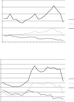
220 |
V. Costantini et al. |
|
|
EPO patents count by country and year, Biopat |
|
||||||||||||||||
6000 |
|
|
|
|
|
|
|
|
|
|
|
|
|
|
|
|
|
|
|
5000 |
|
|
|
|
|
|
|
|
|
|
|
|
|
|
|
|
|
|
|
4000 |
|
|
|
|
|
|
|
|
|
|
|
|
|
|
|
|
|
|
|
3000 |
|
|
|
|
|
|
|
|
|
|
|
|
|
|
|
|
|
|
US |
|
|
|
|
|
|
|
|
|
|
|
|
|
|
|
|
|
|
JP |
|
|
|
|
|
|
|
|
|
|
|
|
|
|
|
|
|
|
|
|
|
2000 |
|
|
|
|
|
|
|
|
|
|
|
|
|
|
|
|
|
|
EU |
1000 |
|
|
|
|
|
|
|
|
|
|
|
|
|
|
|
|
|
|
|
0 |
|
|
|
|
|
|
|
|
|
|
|
|
|
|
|
|
|
|
|
1990 |
1991 |
1992 |
1993 |
1994 |
1995 |
1996 |
1997 |
1998 |
1999 |
2000 |
2001 |
2002 |
2003 |
2004 |
2005 |
2006 |
2007 |
2008 |
2009 |
EPO patents count by country and year, Green Inventoryin BioPat |
|||||||||||||||||||
450 |
|
|
|
|
|
|
|
|
|
|
|
|
|
|
|
|
|
|
|
400 |
|
|
|
|
|
|
|
|
|
|
|
|
|
|
|
|
|
|
|
350 |
|
|
|
|
|
|
|
|
|
|
|
|
|
|
|
|
|
|
|
300 |
|
|
|
|
|
|
|
|
|
|
|
|
|
|
|
|
|
|
|
250 |
|
|
|
|
|
|
|
|
|
|
|
|
|
|
|
|
|
|
US |
200 |
|
|
|
|
|
|
|
|
|
|
|
|
|
|
|
|
|
|
JP |
150 |
|
|
|
|
|
|
|
|
|
|
|
|
|
|
|
|
|
|
EU |
100 |
|
|
|
|
|
|
|
|
|
|
|
|
|
|
|
|
|
|
|
50 |
|
|
|
|
|
|
|
|
|
|
|
|
|
|
|
|
|
|
|
0 |
|
|
|
|
|
|
|
|
|
|
|
|
|
|
|
|
|
|
|
1990 |
1991 |
1992 |
1993 |
1994 |
1995 |
1996 |
1997 |
1998 |
1999 |
2000 |
2001 |
2002 |
2003 |
2004 |
2005 |
2006 |
2007 |
2008 |
2009 |
Fig. 11.3 EPO patents count by country and year, Green Inventory in BioPat and BioPat total
Johnstone et al. (2010) for other green technology domains). Moreover, the effect of the recent economic crisis is clearly visible in the two series.
Finally, Fig. 11.4 shows the patterns of innovation output in the biofuels sector by using all the keywords referring to specific types of raw materials. The food series confirm that old generation biofuels represent more mature technologies, with a high number of patents and more regular performance. In these fields, Japanese patenting activity shows a peak in the 2004 year and a significant decrease later on, whereas USA and EU show a more regular trend and a recent slow decrease. In the sugar series, the three countries seem to have a pretty common trend, with an increase of the patenting activity in the second decade, especially for
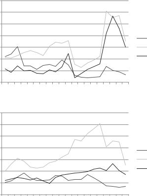
11 BioPat: An Investigation Tool for Analysis of Industry Evolution. . . |
221 |
Japan. In this regard, it is worth reminding that the sugar-based biofuel industries rely on very traditional production process and that the main innovation activity in this field consists in irrigation and agricultural best practices. On the other hand, the two less mature technologies, algae and ligno, show a clear increasing trend after the period 2006/2007, in particular for EU, consistently with the European biofuels policy oriented towards a strong promotion of environmental sustainability standards to be respected in biofuels production process.
Hence, we can conclude that the trend identified in Fig. 11.3 is mainly driven by technologies related to old generation raw material (food), while strong heterogeneity in terms of trends and patents number exists in the dynamics of patenting activities associated with different technology generations.
350 |
|
|
|
|
|
|
|
|
Algae |
|
|
|
|
|
|
|
|
||
300 |
|
|
|
|
|
|
|
|
|
|
|
|
|
|
|
|
|||
|
|
|
|
|
|
|
|
|
|
|
|
|
|
|
|
|
|
|
|
250 |
|
|
|
|
|
|
|
|
|
|
|
|
|
|
|
|
|
|
|
200 |
|
|
|
|
|
|
|
|
|
|
|
|
|
|
|
|
|
|
US |
|
|
|
|
|
|
|
|
|
|
|
|
|
|
|
|
|
|
|
|
150 |
|
|
|
|
|
|
|
|
|
|
|
|
|
|
|
|
|
|
JP |
100 |
|
|
|
|
|
|
|
|
|
|
|
|
|
|
|
|
|
|
EU |
|
|
|
|
|
|
|
|
|
|
|
|
|
|
|
|
|
|
|
|
50 |
|
|
|
|
|
|
|
|
|
|
|
|
|
|
|
|
|
|
|
0 |
|
|
|
|
|
|
|
|
|
|
|
|
|
|
|
|
|
|
|
1990 |
1991 |
1992 |
1993 |
1994 |
1995 |
1996 |
1997 |
1998 |
1999 |
2000 |
2001 |
2002 |
2003 |
2004 |
2005 |
2006 |
2007 |
2008 |
2009 |
700 |
|
|
|
|
|
|
|
|
Food |
|
|
|
|
|
|
|
|
||
600 |
|
|
|
|
|
|
|
|
|
|
|
|
|
|
|
|
|||
|
|
|
|
|
|
|
|
|
|
|
|
|
|
|
|
|
|
|
|
500 |
|
|
|
|
|
|
|
|
|
|
|
|
|
|
|
|
|
|
|
400 |
|
|
|
|
|
|
|
|
|
|
|
|
|
|
|
|
|
|
US |
|
|
|
|
|
|
|
|
|
|
|
|
|
|
|
|
|
|
|
|
300 |
|
|
|
|
|
|
|
|
|
|
|
|
|
|
|
|
|
|
JP |
200 |
|
|
|
|
|
|
|
|
|
|
|
|
|
|
|
|
|
|
EU |
|
|
|
|
|
|
|
|
|
|
|
|
|
|
|
|
|
|
|
|
100 |
|
|
|
|
|
|
|
|
|
|
|
|
|
|
|
|
|
|
|
0 |
|
|
|
|
|
|
|
|
|
|
|
|
|
|
|
|
|
|
|
1990 |
1991 |
1992 |
1993 |
1994 |
1995 |
1996 |
1997 |
1998 |
1999 |
2000 |
2001 |
2002 |
2003 |
2004 |
2005 |
2006 |
2007 |
2008 |
2009 |
Fig. 11.4 Patterns of innovation in the biofuels sector by using all keywords referring to specific raw materials
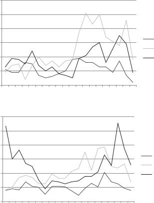
222 |
V. Costantini et al. |
60 |
|
|
|
|
|
|
|
|
Sugar |
|
|
|
|
|
|
|
|
||
|
|
|
|
|
|
|
|
|
|
|
|
|
|
|
|
|
|||
50 |
|
|
|
|
|
|
|
|
|
|
|
|
|
|
|
|
|
|
|
40 |
|
|
|
|
|
|
|
|
|
|
|
|
|
|
|
|
|
|
|
30 |
|
|
|
|
|
|
|
|
|
|
|
|
|
|
|
|
|
|
US |
|
|
|
|
|
|
|
|
|
|
|
|
|
|
|
|
|
|
JP |
|
|
|
|
|
|
|
|
|
|
|
|
|
|
|
|
|
|
|
|
|
20 |
|
|
|
|
|
|
|
|
|
|
|
|
|
|
|
|
|
|
EU |
10 |
|
|
|
|
|
|
|
|
|
|
|
|
|
|
|
|
|
|
|
0 |
|
|
|
|
|
|
|
|
|
|
|
|
|
|
|
|
|
|
|
1990 |
1991 |
1992 |
1993 |
1994 |
1995 |
1996 |
1997 |
1998 |
1999 |
2000 |
2001 |
2002 |
2003 |
2004 |
2005 |
2006 |
2007 |
2008 |
2009 |
120 |
|
|
|
|
|
|
|
Ligno |
|
|
|
|
|
|
|
|
|||
|
|
|
|
|
|
|
|
|
|
|
|
|
|
|
|
||||
100 |
|
|
|
|
|
|
|
|
|
|
|
|
|
|
|
|
|
|
|
80 |
|
|
|
|
|
|
|
|
|
|
|
|
|
|
|
|
|
|
|
60 |
|
|
|
|
|
|
|
|
|
|
|
|
|
|
|
|
|
|
US |
|
|
|
|
|
|
|
|
|
|
|
|
|
|
|
|
|
|
JP |
|
|
|
|
|
|
|
|
|
|
|
|
|
|
|
|
|
|
|
|
|
40 |
|
|
|
|
|
|
|
|
|
|
|
|
|
|
|
|
|
|
EU |
20 |
|
|
|
|
|
|
|
|
|
|
|
|
|
|
|
|
|
|
|
0 |
|
|
|
|
|
|
|
|
|
|
|
|
|
|
|
|
|
|
|
1990 |
1991 |
1992 |
1993 |
1994 |
1995 |
1996 |
1997 |
1998 |
1999 |
2000 |
2001 |
2002 |
2003 |
2004 |
2005 |
2006 |
2007 |
2008 |
2009 |
Fig. 11.4 (continued)
11.5Conclusions
This chapter has analysed issues associated with the measurement of innovation activities through patents in a narrow economic sector such as the biofuels sector. The proposed methodology aims to solve some of the drawbacks related to how patent data are allocated and organised in international databases.
In order to create a database which includes patents strictly related to the investigated field, we developed an original method based on keywords, rather than on International Patent Classification (IPC) codes. Starting with a systematic mapping of biofuel production processes, we built a simplified but comprehensive description of technological domains related to the production of biofuels by applying the so-called process analysis. The keyword selection is based on
11 BioPat: An Investigation Tool for Analysis of Industry Evolution. . . |
223 |
an iterative approach based on the analysis of recent scientific literature. The construction of the database allows a distinction to be made between innovations in raw materials and transformation processes. Moreover, both materials and processes were divided into first generation and new generation, as well as according to the biofuel type. The database was finalised by a series of interviews with experts in biofuels and compared with IPC-based biofuel codes, revealing improved accuracy when selecting data using our methodology.
Our preliminary descriptive findings show that the distinction between different technology generations can provide interesting insights into the evolution of technologies in the biofuels sector. Moreover, the information contained in the database will allow in depth scrutiny of the characteristics, determinants and effects of innovative activities in this sector. In particular, the possibility of constructing indicators that capture the dynamics of patenting activities, their value and their concentration in terms of geographical location, holding companies and inventors will allow better comprehension of the sectoral innovation system that is being examined.
Acknowledgments The authors would like to thank Alessandra Molina and Alessandro Palma for their initial contribution during the collection of keywords, Federico Caviggioli for his advice on downloading patents, Vincenzo Alfano, Alessandro Blasi and Carlo Pignatelli for patent validation and Carlotta Greci and Corrado Pollastri for assistance in data management. The support of the Regione Lazio, University Roma Tre, INEA, ENEA and European Union D.G. Research with the grant number 266959 to the research project “PICK-ME – Policy Incentives for the Creation of Knowledge: Methods and Evidence” is also gratefully acknowledged. The usual disclaimers apply.

224 V. Costantini et al.
Appendix
Table 11.7 Examples of keywords
|
Eicosapentaenoic acid |
|
Fame |
scenedesmus |
Peanut |
|
|
|
Fatty acid methyl esters |
Corn |
Oil-bearing organisms |
Fatty acid ethyl esters |
Maize |
Jatropha curcas |
Free fatty acid |
Cassava |
Jatropha |
Lipids as feedstock |
Grain |
Babassu coconut |
Lipids microbial organisms |
Soybean |
Helianthus tuberosus |
Fatty acyl-ACP thioesterase |
Genetically engineered microbes |
Oleaginous microorganisms |
Fatty acyl-CoA/aldehyde |
Genetically modified crops |
Rhodotorula glutinis |
reductase |
|
|
Fatty aldehyde decarbonylase |
Lignocellulosic |
Medicago sativa L. |
Acyl carrier protein |
Perennial grasses |
Nut shells |
Volatile fatty acids |
Forest |
Sugar cane |
Microbial lipids |
Panicum virgatum L. |
Beet |
Microbial hosts |
Perennial plant |
Sorghum |
Trichosporon |
Phalaris |
Sugar esters |
Agricultural feedstocks |
Alfalfa |
Bagasse |
Starch |
Reed canary grass |
Fermentable sugars |
Corncobs |
Fibrous plant materials |
Cooking oil |
Corn stover |
Switchgrass |
Wet organic wastes |
Cereal straw |
Bark |
Monosodium glutamate |
|
|
wastewater |
Forest harvest residues |
Wood shavings |
Urban wood residues |
Husks |
Chipboards |
Ammonium |
Chlorella vulgaris |
Garden mulch |
Animal waste |
Spirulina maxima |
Vegetative grasses |
Anlage |
Nannochloropsis sp. |
Miscanthus |
Excreta |
Scenedesmus obliquus |
Prairie grass |
Feed mixture |
Dunaliella tertiolecta |
Short rotation forest species |
Fibrobacter succinogenes |
Scenedesmus dimorphus |
Eucalyptus |
Kalium |
Chlorella emersonii |
Poplars |
Lignocellulose |
Chlorella protothecoides |
Lignin |
Liquid manure |
Chlorella minutissima |
Cellulose |
Microorganisms |
Dunaliella bioculata |
Hemicellulose |
Ruminococcus albus |
Dunaliella salina |
Wood process residues |
Sewage |
Microalgae oil |
Wheat chaff |
Siloxane |
Phaeodactylum tricornutum |
Animal fat |
Sulphide |
Vegetable oil |
Edible tallow |
Digested sludge |
Soya oil |
Animal manure |
Fibrous material |
Untreated raw oils |
Granular sludge |
Hydrolysate |
Oilseed rape |
Porcine pancreatic lipase |
Liquid manure |
Coconut oil |
Rapeseed |
Mesophilic bacteria |
Jojoba (limited to biodiesel) |
Palm oil |
Microbial consortia |
Canola oil (limited to biodiesel) |
Organic material |
Sludge |
Methanogenic bacteria |
Animal slurries |
Treated wastewater |
|
|
|
11 BioPat: An Investigation Tool for Analysis of Industry Evolution. . . |
225 |
References
Archibugi, D., & Pianta, M. (1996). Measuring technological through patents and innovation surveys. Technovation, 16(9), 451–468.
Corrocher, N., Malerba, F., & Montobbio, F. (2007). Schumpeterian patterns of innovative activity in the ICT field. Research Policy, 36(3), 418–432.
Costantini, V., & Crespi, F. (2012). Public policies for a sustainable energy sector: Regulation, diversity and fostering of innovation. Journal of Evolutionary Economics. doi:10.1007/ s00191-010-0211-3.
Coulter, N., et al. (1998). Software engineering as seen through its research literature: A study in co-word analysis. Journal of the American Society for Information Science, 49(13), 1206–1223.
De Looze, M.-A., & Lemarie, J. (1997). Corpus relevance through co-word analysis: An application to plant proteins. Scientometrics, 39(3), 267–280.
EC. (2005, December 7). Biomass action plan (COM(2005) 628 final). Brussels. http://europa.eu/ legislation_summaries/energy/renewable_energy/l27014_en.htm
EC. (2006, February 8). European Union biofuel strategy (COM(2006) 34 final). Brussels. http:// europa.eu/legislation_summaries/internal_market/single_market_for_goods/motor_vehicles/ interactions_industry_policies/l28175_en.htm
EC. (2007, January 10). Renewable energy roadmap (COM(2006) 848 final). Brussels. http:// europa.eu/legislation_summaries/energy/renewable_energy/l27065_en.htm
EUROSTAT. (2007). Energy, transport and environment indicators. Luxemburg: Eurostat Pocketbooks.
Griliches, Z. (1990). Patent statistics as economic indicators: A survey. Journal of Economic Literature, XXVIII, 1661–1707.
Hekkert, M. P., Suurs, R. A. A., Negro, S. O., Kuhlmann, S., & Smits, R. E. H. M. (2007). Functions of innovation systems: A new approach for analyzing technological change.
Technological Forecasting and Social Change, 74, 413–432. IEA. (2007). World energy outlook 2007. Paris: IEA.
IEA. (2008). From 1st to 2nd generation biofuels technologies. An overview of current industry and R&D activities. Paris: IEA.
IPC Guide. (2011). Available at http://www.wipo.int/export/sites/www/classifications/ipc/en/ guide/guide_ipc.pdf
Jaffe, A. B., & Trajtenberg, M. (2002). Patents, citations and innovations. Cambridge: The MIT Press.
Jaffe, A. B., Trajtenberg, M., & Henderson, R. (1993). Geographic localisation of knowledge spillovers as evidenced by patent citations. Quarterly Journal of Economics, 108, 577–598.
Johnstone, N., Hasˇcˇicˇ, I., & Popp, D. (2010). Renewable energy policies and technological innovation: Evidence based on patent counts. Environmental and Resource Economics, 45(1), 133–155.
Karmarkar-Deshmukh, R., & Pray, C. E. (2009). Private sector innovation in biofuels in the United States: Induced by prices or policies? AgBioforum, 12(1), 141–148.
Lemley, M., & Sampat, B. N. (2008). Examiner characteristics and the patent grant rate. (Stanford Law and Economics Olin Working Paper No. 369). http://papers.ssrn.com/sol3/ papers.cfm?abstract_id¼1329091
Narin, F., Hamilton, K. S., & Olivastro, D. (1997). The increasing linkage between U.S. technology and public science. Research Policy, 26(3), 317–330.
OECD-FAO. (2010). Agricultural outlook 2010–2019. Paris: OECD-FAO.
Picci, L. (2010). The internationalization of inventive activity: A gravity model using patent data.
Research Policy, 39, 1070–1081.
Sirilli, G. (1997). Science and technology indicators: The state of the art and prospects for the future. In G. Antonelli & N. De Liso (Eds.), Economics of structural and technological change. London: Routledge.
226 |
V. Costantini et al. |
The Economist. (2011, March 17). Patent reform: The spluttering invention machine – America’s patent system has problems; a new law would fix only a few.
UNCTAD-ICTSD. (2005). Resource book on TRIPS and development. New York: Cambridge University Press.
UNEP. (2010, July). Global trends in green energy 2009: New power capacity from renewable sources tops fossil fuels again in US, Europe. Press release
Weitzman, M. L. (1996). Hybridizing growth theory. American Economic Review, 86, 207–212. Weitzman, M. L. (1998). Recombinant growth. Quarterly Journal of Economics, 113, 331–360.