The Official Guide to Learning OpenGL, Version 1.1 (Redbook Second Edition)

OpenGL Programming Guide (Addison-Wesley Publishing Company)

void glutIdleFunc(void (*func)(void));

Specifies the function, func, to be executed if no other events are pending. If NULL (zero) is passed in, execution of func is disabled.

Running the Program

After all the setup is completed, GLUT programs enter an event processing loop, glutMainLoop().

void glutMainLoop(void);

Enters the GLUT processing loop, never to return. Registered callback functions will be called when the corresponding events instigate them.

OpenGL Programming Guide (Addison-Wesley Publishing Company)

http://heron.cc.ukans.edu/ebt-bin/nph-dweb/dynaw...Generic__BookTextView/36440;cs=fullhtml;pt=34575 (5 of 5) [4/28/2000 9:51:12 PM]

OpenGL Programming Guide (Addison-Wesley Publishing Company)

OpenGL Programming Guide (Addison-Wesley Publishing Company)

Appendix E

Calculating Normal Vectors

This appendix describes how to calculate normal vectors for surfaces. You need to define normals to use the OpenGL lighting facility, which is described in Chapter 5. "Normal Vectors" in Chapter 2 introduces normals and the OpenGL command for specifying them. This appendix goes through the details of calculating them. It has the following major sections:

●"Finding Normals for Analytic Surfaces"

●"Finding Normals from Polygonal Data"

Since normals are perpendicular to a surface, you can find the normal at a particular point on a surface by first finding the flat plane that just touches the surface at that point. The normal is the vector that's perpendicular to that plane. On a perfect sphere, for example, the normal at a point on the surface is in the same direction as the vector from the center of the sphere to that point. For other types of surfaces, there are other, better means for determining the normals, depending on how the surface is specified.

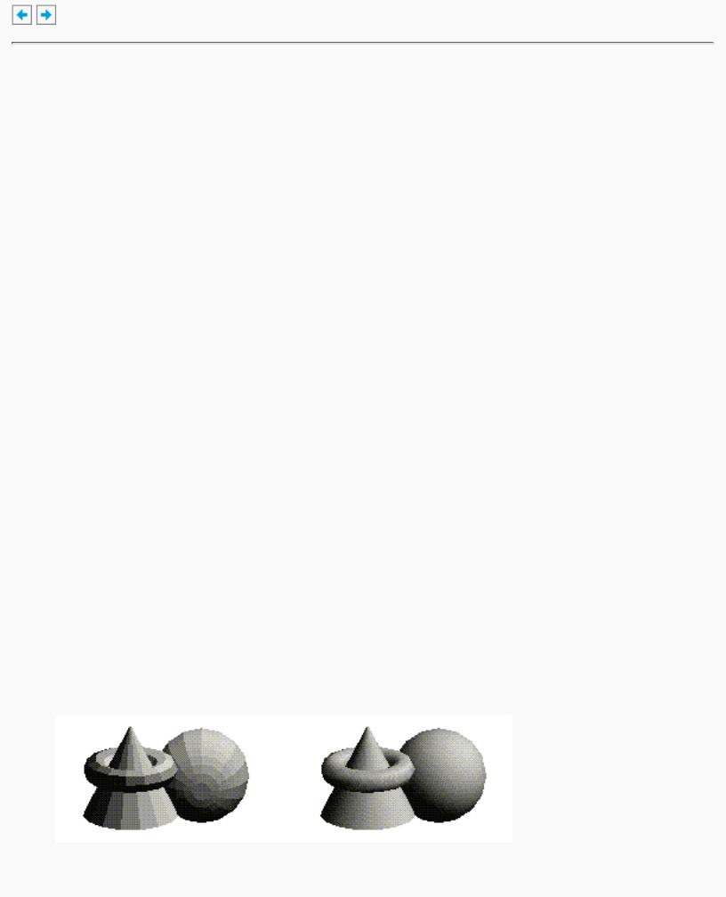
Recall that smooth curved surfaces are approximated by a large number of small flat polygons. If the vectors perpendicular to these polygons are used as the surface normals in such an approximation, the surface appears faceted, since the normal direction is discontinuous across the polygonal boundaries. In many cases, however, an exact mathematical description exists for the surface, and true surface normals can be calculated at every point. Using the true normals improves the rendering considerably, as shown in Figure E-1. Even if you don't have a mathematical description, you can do better than the faceted look shown in the figure. The two major sections in this appendix describe how to calculate normal vectors for these two cases:

●"Finding Normals for Analytic Surfaces" explains what to do when you have a mathematical description of a surface.

●"Finding Normals from Polygonal Data" covers the case when you have only the polygonal data to describe a surface.

Figure E-1 : Rendering with Polygonal Normals vs. True Normals

http://heron.cc.ukans.edu/ebt-bin/nph-dweb/dynaw...Generic__BookTextView/37099;cs=fullhtml;pt=36440 (1 of 5) [4/28/2000 9:51:24 PM]

OpenGL Programming Guide (Addison-Wesley Publishing Company)

Finding Normals for Analytic Surfaces

Analytic surfaces are smooth, differentiable surfaces that are described by a mathematical equation (or set of equations). In many cases, the easiest surfaces to find normals for are analytic surfaces for which you have an explicit definition in the following form:

V(s,t) = [ X(s,t) Y(s,t) Z(s,t) ]

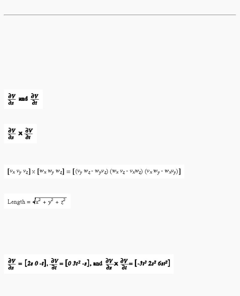
where s and t are constrained to be in some domain, and X, Y, and Z are differentiable functions of two variables. To calculate the normal, find

which are vectors tangent to the surface in the s and t directions. The cross product

is perpendicular to both and, hence, to the surface. The following shows how to calculate the cross product of two vectors. (Watch out for the degenerate cases where the cross product has zero length!)

You should probably normalize the resulting vector. To normalize a vector [x y z], calculate its length

and divide each component of the vector by the length.

As an example of these calculations, consider the analytic surface

V(s,t) = [ s2 t3 3-st ]

From this we have

So, for example, when s=1 and t=2, the corresponding point on the surface is (1, 8, 1), and the vector

http://heron.cc.ukans.edu/ebt-bin/nph-dweb/dynaw...Generic__BookTextView/37099;cs=fullhtml;pt=36440 (2 of 5) [4/28/2000 9:51:24 PM]

OpenGL Programming Guide (Addison-Wesley Publishing Company)

(-24, 2, 24) is perpendicular to the surface at that point. The length of this vector is 34, so the unit normal vector is (-24/34, 2/34, 24/34) = (-0.70588, 0.058823, 0.70588).

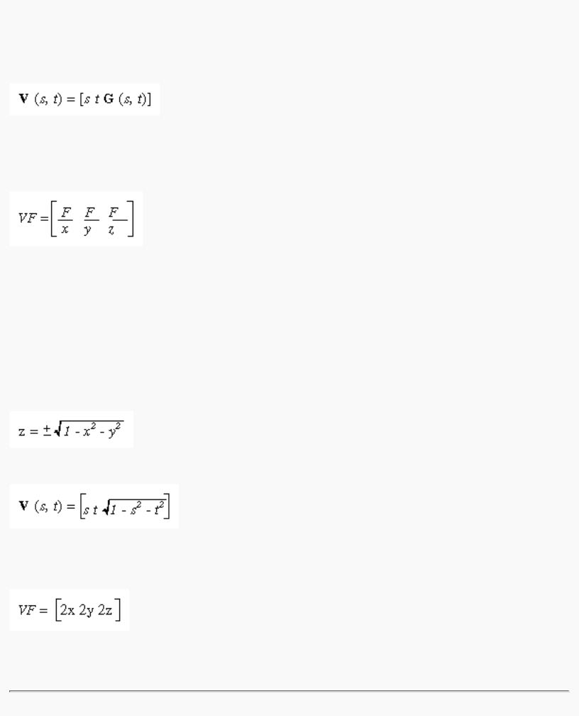
For analytic surfaces that are described implicitly, as F(x, y, z) = 0, the problem is harder. In some cases, you can solve for one of the variables, say z = G(x, y), and put it in the explicit form given previously:

Then continue as described earlier.

If you can't get the surface equation in an explicit form, you might be able to make use of the fact that the normal vector is given by the gradient

evaluated at a particular point (x, y, z). Calculating the gradient might be easy, but finding a point that lies on the surface can be difficult. As an example of an implicitly defined analytic function, consider the equation of a sphere of radius 1 centered at the origin:

x2 + y2 + z2 - 1 = 0 )

This means that

F (x, y, z) = x2 + y2 + z2 - 1

which can be solved for z to yield

Thus, normals can be calculated from the explicit form

as described previously.

If you could not solve for z, you could have used the gradient

as long as you could find a point on the surface. In this case, it's not so hard to find a point - for example, (2/3, 1/3, 2/3) lies on the surface. Using the gradient, the normal at this point is (4/3, 2/3, 4/3). The unit-length normal is (2/3, 1/3, 2/3), which is the same as the point on the surface, as expected.

http://heron.cc.ukans.edu/ebt-bin/nph-dweb/dynaw...Generic__BookTextView/37099;cs=fullhtml;pt=36440 (3 of 5) [4/28/2000 9:51:24 PM]

OpenGL Programming Guide (Addison-Wesley Publishing Company)

Finding Normals from Polygonal Data

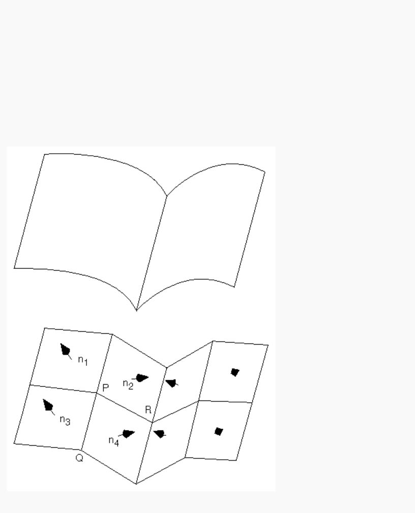
As mentioned previously, you often want to find normals for surfaces that are described with polygonal data such that the surfaces appear smooth rather than faceted. In most cases, the easiest way for you to do this (though it might not be the most efficient way) is to calculate the normal vectors for each of the polygonal facets and then to average the normals for neighboring facets. Use the averaged normal for the vertex that the neighboring facets have in common. Figure E-2 shows a surface and its polygonal approximation. (Of course, if the polygons represent the exact surface and aren't merely an approximation - if you're drawing a cube or a cut diamond, for example - don't do the averaging. Calculate the normal for each facet as described in the following paragraphs, and use that same normal for each vertex of the facet.)

http://heron.cc.ukans.edu/ebt-bin/nph-dweb/dynaw...Generic__BookTextView/37099;cs=fullhtml;pt=36440 (4 of 5) [4/28/2000 9:51:24 PM]

OpenGL Programming Guide (Addison-Wesley Publishing Company)

Figure E-2 : Averaging Normal Vectors

To find the normal for a flat polygon, take any three vertices v1, v2, and v3 of the polygon that do not lie in a straight line. The cross product

[v1 - v2] × [v2 - v3]

is perpendicular to the polygon. (Typically, you want to normalize the resulting vector.) Then you need to average the normals for adjoining facets to avoid giving too much weight to one of them. For instance, in the example shown in Figure E-2, if n1, n2, n3, and n4 are the normals for the four polygons meeting at point P, calculate n1+n2+n3+n4 and then normalize it. (You can get a better average if you weight the normals by the size of the angles at the shared intersection.) The resulting vector can be used as the normal for point P.

Sometimes, you need to vary this method for particular situations. For instance, at the boundary of a surface (for example, point Q in Figure E-2), you might be able to choose a better normal based on your knowledge of what the surface should look like. Sometimes the best you can do is to average the polygon normals on the boundary as well. Similarly, some models have some smooth parts and some sharp corners (point R is on such an edge in Figure E-2). In this case, the normals on either side of the crease shouldn't be averaged. Instead, polygons on one side of the crease should be drawn with one normal, and polygons on the other side with another.

OpenGL Programming Guide (Addison-Wesley Publishing Company)

http://heron.cc.ukans.edu/ebt-bin/nph-dweb/dynaw...Generic__BookTextView/37099;cs=fullhtml;pt=36440 (5 of 5) [4/28/2000 9:51:24 PM]

OpenGL Programming Guide (Addison-Wesley Publishing Company)

OpenGL Programming Guide (Addison-Wesley Publishing Company)

Appendix F

Homogeneous Coordinates and

Transformation Matrices

This appendix presents a brief discussion of homogeneous coordinates. It also lists the form of the transformation matrices used for rotation, scaling, translation, perspective projection, and orthographic projection. These topics are introduced and discussed in Chapter 3. For a more detailed discussion of these subjects, see almost any book on three-dimensional computer graphics - for example, Computer Graphics: Principles and Practice by Foley, van Dam, Feiner, and Hughes (Reading, MA: Addison-Wesley, 1990) - or a text on projective geometry - for example, The Real Projective Plane, by H. S. M. Coxeter, 2nd ed. (Cambridge: Cambridge University Press, 1961). In the discussion that follows, the term homogeneous coordinates always means three-dimensional homogeneous coordinates, although projective geometries exist for all dimensions.

This appendix has the following major sections:

●"Homogeneous Coordinates"

●"Transformation Matrices"

Homogeneous Coordinates

OpenGL commands usually deal with twoand three-dimensional vertices, but in fact all are treated internally as three-dimensional homogeneous vertices comprising four coordinates. Every column vector (x, y, z, w)T represents a homogeneous vertex if at least one of its elements is nonzero. If the real number a is nonzero, then (x, y, z, w)T and (ax, ay, az, aw)T represent the same homogeneous vertex. (This is just like fractions: x/y = (ax)/(ay).) A three-dimensional euclidean space point (x, y, z)T becomes the homogeneous vertex with coordinates (x, y, z, 1.0)T, and the two-dimensional euclidean point (x, y)T becomes (x, y, 0.0, 1.0)T.

As long as w is nonzero, the homogeneous vertex (x, y, z, w)T corresponds to the three-dimensional point (x/w, y/w, z/w)T. If w = 0.0, it corresponds to no euclidean point, but rather to some idealized "point at infinity." To understand this point at infinity, consider the point (1, 2, 0, 0), and note that the sequence of points (1, 2, 0, 1), (1, 2, 0, 0.01), and (1, 2.0, 0.0, 0.0001), corresponds to the euclidean points (1, 2), (100, 200), and (10000, 20000). This sequence represents points rapidly moving toward infinity along the line 2x = y. Thus, you can think of (1, 2, 0, 0) as the point at infinity in the direction of that line.

http://heron.cc.ukans.edu/ebt-bin/nph-dweb/dynaw...Generic__BookTextView/37451;cs=fullhtml;pt=37099 (1 of 5) [4/28/2000 9:51:52 PM]

OpenGL Programming Guide (Addison-Wesley Publishing Company)

Note: OpenGL might not handle homogeneous clip coordinates with w < 0 correctly. To be sure that your code is portable to all OpenGL systems, use only nonnegative w values.

Transforming Vertices

Vertex transformations (such as rotations, translations, scaling, and shearing) and projections (such as perspective and orthographic) can all be represented by applying an appropriate 4 × 4 matrix to the coordinates representing the vertex. If v represents a homogeneous vertex and M is a 4 × 4 transformation matrix, then Mv is the image of v under the transformation by M. (In computer-graphics applications, the transformations used are usually nonsingular - in other words, the matrix M can be inverted. This isn't required, but some problems arise with nonsingular transformations.)

After transformation, all transformed vertices are clipped so that x, y, and z are in the range [- &ohgr; , w] (assuming w > 0). Note that this range corresponds in euclidean space to [-1.0, 1.0].

Transforming Normals

Normal vectors aren't transformed in the same way as vertices or position vectors. Mathematically, it's better to think of normal vectors not as vectors, but as planes perpendicular to those vectors. Then, the transformation rules for normal vectors are described by the transformation rules for perpendicular planes.

A homogeneous plane is denoted by the row vector (a, b, c, d), where at least one of a, b, c, or d is nonzero. If q is a nonzero real number, then (a, b, c, d) and (qa, qb, qc, qd) represent the same plane. A point (x, y, z, w)T is on the plane (a, b, c, d) if ax+by+cz+dw = 0. (If w = 1, this is the standard description of a euclidean plane.) In order for (a, b, c, d) to represent a euclidean plane, at least one of a, b, or c must be nonzero. If they're all zero, then (0, 0, 0, d) represents the "plane at infinity," which contains all the "points at infinity."

If p is a homogeneous plane and v is a homogeneous vertex, then the statement "v lies on plane p" is written mathematically as pv = 0, where pv is normal matrix multiplication. If M is a nonsingular vertex transformation (that is, a 4 × 4 matrix that has an inverse M-1), then pv = 0 is equivalent to pM-1Mv = 0, so Mv lies on the plane pM-1. Thus, pM-1 is the image of the plane under the vertex transformation

M.

If you like to think of normal vectors as vectors instead of as the planes perpendicular to them, let v and n be vectors such that v is perpendicular to n. Then, nTv = 0. Thus, for an arbitrary nonsingular transformation M, nTM-1Mv = 0, which means that nTM-1 is the transpose of the transformed normal vector. Thus, the transformed normal vector is (M-1)Tn. In other words, normal vectors are transformed by the inverse transpose of the transformation that transforms points. Whew!

Transformation Matrices

Although any nonsingular matrix M represents a valid projective transformation, a few special matrices are particularly useful. These matrices are listed in the following subsections.

http://heron.cc.ukans.edu/ebt-bin/nph-dweb/dynaw...Generic__BookTextView/37451;cs=fullhtml;pt=37099 (2 of 5) [4/28/2000 9:51:52 PM]

OpenGL Programming Guide (Addison-Wesley Publishing Company)

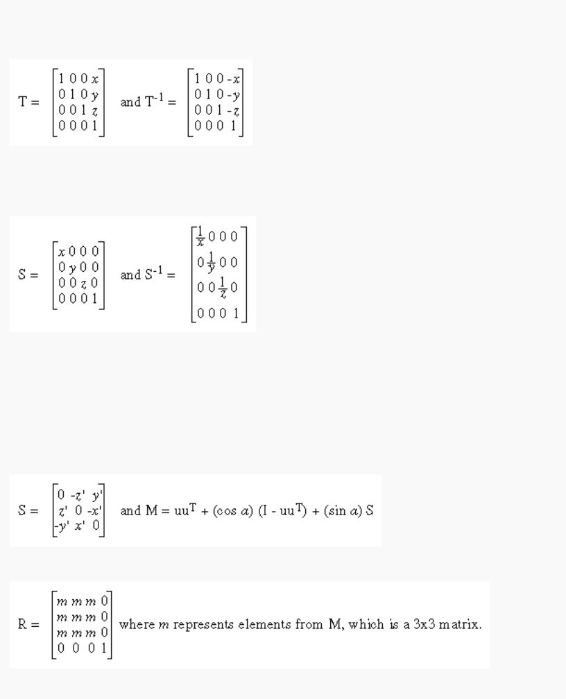
Translation

The call glTranslate*(x, y, z) generates T, where

Scaling

The call glScale*(x, y, z) generates S, where

Notice that S-1 is defined only if x, y, and z are all nonzero.

Rotation

The call glRotate*(a, x, y, z) generates R as follows: Let v = (x, y, z)T, and u = v/||v|| = (x', y', z')T.

Also let

Then

http://heron.cc.ukans.edu/ebt-bin/nph-dweb/dynaw...Generic__BookTextView/37451;cs=fullhtml;pt=37099 (3 of 5) [4/28/2000 9:51:52 PM]

OpenGL Programming Guide (Addison-Wesley Publishing Company)

The R matrix is always defined. If x=y=z=0, then R is the identity matrix. You can obtain the inverse of R, R-1, by substituting - &agr; for a, or by transposition.

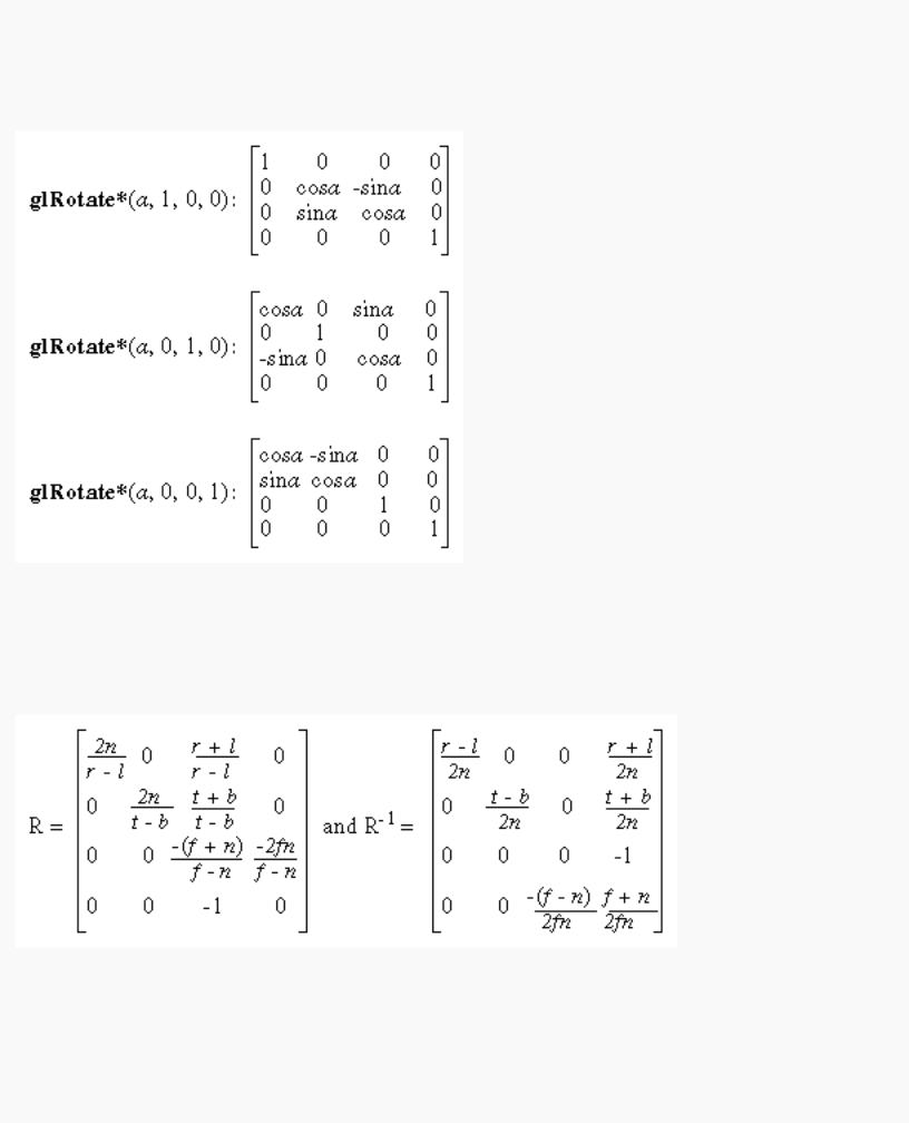
The glRotate*() command generates a matrix for rotation about an arbitrary axis. Often, you're rotating about one of the coordinate axes; the corresponding matrices are as follows:

As before, the inverses are obtained by transposition.

Perspective Projection

The call glFrustum(l, r, b, t, n, f) generates R, where

R is defined as long as l ≠ r, t ≠ b, and n ≠ f.

http://heron.cc.ukans.edu/ebt-bin/nph-dweb/dynaw...Generic__BookTextView/37451;cs=fullhtml;pt=37099 (4 of 5) [4/28/2000 9:51:52 PM]