The Carnot Refrigerator

Because each step in the Carnot cycle is reversible, the entire cycle may be reversed, converting the engine into a refrigerator. The coefficient of performance of the Carnot refrigerator is obtained by combining the general definition of , , with Eq. (46) for the Carnot cycle. We first rewrite

Then we substitute Eq. (46), , into this expression. The result is

(coefficient of performance of a Carnot refrigerator) (20.15)

When the temperature difference is small, is much larger than unity; in this case a lot of heat can be "pumped" from the lower to the higher temperature with only a little expenditure of work. But the greater the temperature difference, the smaller the value of and the more work is required to transfer a given quantity of heat.

Example 20.4 Analyzing a Carnot refrigerator If the cycle described in Example 20.3 is run backward as a refrigerator, what is its coefficient of performance?

Solution This problem uses the ideas as for refrigerators in general as well as the above discussion of Carnot refrigerators. Equation (20.9) gives the coefficient of performance of any refrigerator in terms of the heat extracted from the cold reservoir per cycle and the work that must be done per cycle. In Example 20.3 we found that in one cycle the Carnot engine rejects heat = -345 J to the cold reservoir and does work = 230 J. Hence, when run in reverse as a refrigerator, the system extracts heat = +345 J from the cold reservoir while requiring a work input of = - 230 J. From Eq. ,

Because the cycle is a Carnot cycle, we may also use Eq. (20.15):

EVALUATE: For a Carnot cycle, and depend only on the tem­peratures, as shown by Eqs. (20.14) and (20.15), and we don't need to calculate Q and W. For cycles containing irreversible processes, however, these two equations are not valid, and more detailed calculations are necessary.

Entropy

The second law of thermodynamics, as we have stated it, is rather different in form from many familiar physical laws. It is not an equation or a quantitative relationship but rather a statement of impossibility. However, the second law can be stated as a quantitative relationship with the concept of entropy, the subject of this section.

Entropy and Disorder

We have talked about several processes that proceed naturally in the direction of increasing disorder. Irreversible heat flow increases disorder because the molecules are initially sorted into hotter and cooler regions; this sorting is lost when the system comes to thermal equilibrium. Adding heat to a body increases its disorder because it increases average molecular speeds and therefore the randomness of molecular motion. Free expansion of a gas increases its disorder because the molecules have greater randomness of position after the expansion than before.

Entropy provides a quantitative measure of disorder. To introduce this concept, let's consider an infinitesimal isothermal expansion of an ideal gas. We add heat and let the gas expand just enough to keep the temperature constant. Because the internal energy of an ideal gas depends only on its temperature, the internal energy is also constant; thus from the first law, the work done by the gas is equal to the heat added. That is,

so .

The gas is in a more disordered state after the expansion than before because the molecules are moving in a larger volume and have more randomness of position. Thus the fractional volume change is a measure of the increase in disorder, and the above equation shows that it is proportional to the quantity . We introduce the symbol for the entropy of the system, and we define the infinitesimal entropy change during an infinitesimal reversible process at absolute temperature as

(infinitesimal reversible process) (20.17).

If a total amount of heat is added during a reversible isothermal process at absolute temperature , the total entropy change is given by

(20.18).

Entropy has units of energy divided by temperature; the SI unit of entropy is 1 J/K. We can see how the quotient is related to the increase in disorder. Higher temperature means greater randomness of motion. If the substance is initially cold, with little molecular motion, adding heat causes a substantial fractional increase in molecular motion and randomness. But if the substance is already hot, the same quantity of heat adds relatively little to the greater molecular motion already present. So the quotient is an appropriate characterization of the increase in randomness or disorder when heat flows into a system.

Example 20.5 Entropy change in melting

One kilogram of ice at 0°C is melted and converted to water at 0°C. Compute its change in entropy, assuming that the melting is done reversibly. The heat of fusion of water is = 3.34 X 10⁵j/kg.

Solution The melting occurs at a constant temperature of 0°C, so this is a reversible isothermal process. We are given the amount of heat added (in terms of the heat of fusion) and the temperature = 273 K. (Note that in entropy calculations we must always use absolute, or Kelvin, temperatures.) We can then calculate the entropy change using Eq. (20.18). We are given the amount of heat added (in terms of the heat of fusion) and the temperature K. we can then calculate the entropy change using Eq/(20.18)

Fig. 20.18

EXECUTE: The heat needed to melt the ice is = 3.34 X 10⁵ J. From Eq. (20.18) the increase in entropy of the system is

J/K.

This increase corresponds to the increase in disorder when the water molecules go from the highly ordered state of a crystalline solid to the much more disordered state of a liquid (Fig. 20.18).

In any isothermal reversible process, the entropy change equals the heat transferred divided by the absolute temperature. When we refreeze the water, has the opposite sign, and the entropy change of the water is = -1.22 X 10³ J/K. The water molecules rearrange themselves into a crystal to form ice, so disorder and entropy both decrease.

Entropy in Reversible Processes

We can generalize the definition of entropy change to include any reversible process leading from one state to another, whether it is isothermal or not. We represent the process as a series of infinitesimal reversible steps. During a typical step, an infinitesimal quantity of heat is added to the system at absolute temperature . Then we sum (integrate) the quotients for the entire process; that is,

(20.19)

The limits 1 and 2 refer to the initial and final states.

Because entropy is a measure of the disorder of a system in any specific state, it must depend only on the current state of the system, not on its past history. We will show later that this is indeed the case. When a system proceeds from an initial state with entropy to a final state with entropy , the change in entropy defined by Eq. (20.19) does not depend on the path leading from the initial to the final state but is the same for all possible processes leading from state 1 to state 2. Thus the entropy of a system must also have a definite value for any given state of the system. We recall that internal energy, also has this property, although entropy and internal energy are very different quantities.

Since entropy is a function only of the state of a system, we can also compute entropy changes in irreversible (nonequilibrium) processes for which Eqs. (20.17) and (20.19) are not applicable. We simply invent a path connecting the given initial and final states that does consist entirely of reversible equilibrium processes and compute the total entropy change for that path. It is not the actual path, but the entropy change must be the same as for the actual path.

As with internal energy, the above discussion does not tell us how to calculate entropy itself, but only the change in entropy in any given process. Just as with internal energy, we may arbitrarily assign a value to the entropy of a system in a specified reference state and then calculate the entropy of any other state with reference to this.

Example 20.6 Entropy change in a temperature change One kilogram of water at 0°C is heated to 100°C. Compute its change in entropy.

Solution In practice, the process described would be done irreversibly, perhaps by setting a pan of water on an electric range whose cooking surface is maintained at 100°C. But the entropy change of the water depends only on the initial and final states of the system, and is the same whether the process is reversible or irreversible. We can imagine that the temperature of the water is increased reversibly in a series of infinitesimal steps, in each of which the temperature is raised by an infinitesimal amount . We then use Eq. (20.19) to integrate over all these steps and calculate the entropy change for the total process.

The heat required to carry out each such infinitesimal step is . Substituting this into Eq. (20.19) and integrating, we find

The entropy change is positive, as it must be for a process in which the system absorbs heat.

In this calculation we assumed that the specific heat doesn't depend on temperature. That's a pretty good approximation, since for water increases by only 1% between 0°C and 100°C.

CAUTION When can (and cannot) be used. In solving this problem you might be tempted to avoid doing an integral by using the simpler expression in Eq. (20.18), . This would be incorrect, however, because Eq. (20.18) is applicable only to isothermal processes, and the initial and final temperatures in our example are not the same. The only correct way to find the entropy change in a process with different initial and final temperatures is to use Eq. (20.19).

Example 20.7 A reversible adiabatic process

A gas expands adiabatically and reversibly. What is its change in entropy?

Solution In an adiabatic process, no heat enters or leaves the system. Hence and there is no change in entropy in this reversible process: . Every reversible adiabatic process is a constant-entropy process. (For this reason, reversible adiabatic processes are also called isentropic processes.) The increase in disorder resulting from the gas occupying a greater volume is exactly balanced by the decrease in disorder associated with the lowered temperature and reduced molecular speeds.

Example 20.8 Entropy change in a free expansion

A thermally insulated box is divided by a partition into two compartments, each having volume . (Fig. 20.19). Initially, one compartment contains moles of an ideal gas at temperature , and the other compartment is evacuated. We then break the partition, and the gas expands to fill both compartments. What is the entropy change in this free-expansion process?

Solution For this process, , , , and therefore (because the system is an ideal gas) . We might think that the entropy change is zero because there is no heat exchange. But Eq. (20.19) can be used to calculate entropy changes for reversible processes only; this free expansion is not reversible, and there is an entropy change. The process is adiabatic because , but it is not isentropic because . As we mentioned at the beginning of this section, entropy increases in a free expansion because the positions of the molecules are more random than before the expansion.

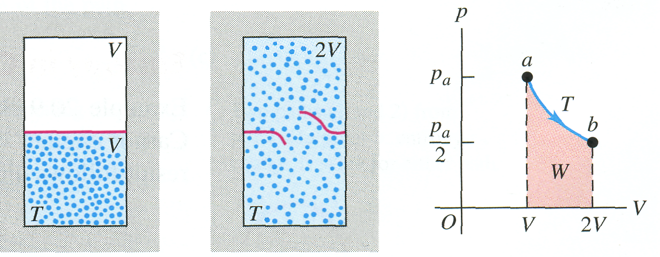
20.19 (a,b) Free expansion of an insulated ideal gas. (c) The free-expansion process doesn't pass through equilibrium states from a to b. However, the entropy change S_b - S_a can be calculated by using the isothermal path shown or any reversible path from a to b.

To calculate , we recall that the entropy change depends only on the initial and final states. We can devise a reversible process having the same endpoints, use Eq. (20.19) to calculate its entropy change, and thus determine the entropy change in the original process. An appropriate reversible process in this case is an isothermal expansion from to at temperature . The gas does work W during this substitute expansion, so an equal amount of heat Q must be supplied to keep the internal energy constant. We find the entropy change for this reversible isothermal process using Eq. (20.18); the entropy change for the free expansion will be the same.

The work done by n moles of ideal gas in an isothermal expansion from , to is . Using and , we have

Thus the entropy change is

which is also the entropy change for the free expansion with the same initial and final states. For 1 mole,

J/K

EVALUATE: The entropy change is positive, as we predicted. The factor ( ) in our answer is a result of the volume having increased by a factor of 2. Can you show that if the volume had increased in the free expansion from to , where is an arbitrary number, the entropy change would have been ?

Example 20.9 Entropy and the Carnot cycle For the Carnot engine in Example 20.2 (Section 20.6), find the total entropy change in the engine during one cycle.

Solution All four steps in the Carnot cycle are reversible (see Fig. 20.13), so we can use the expression for the change in entropy in a reversible process. We find the entropy change for each step and then add the entropy changes to get the total for the cycle as a whole.

EXECUTE: There is no entropy change during the adiabatic expansion or adiabatic compression. During the isothermal expansion at = 500 K the engine takes in 2000 J of heat, and its entropy change, from Eq. (20.18), is

.

During the isothermal compression at = 350 K the engine gives off 1400 J of heat, and its entropy change is

The total entropy change in the engine during one cycle is 4.0 J/K + (-4.0 j/K) = 0.

EVALUATE: The result tells us that when the Carnot engine completes a cycle, it has the same entropy as it did at the beginning of the cycle. We'll explore this result in the following subsection.

What is the total entropy change of the engine's environment during this cycle? The hot (500 K) reservoir gives off 2000 J of heat during the reversible isothermal expansion, so its entropy change is (-2000J)/(500K) = -4.0 j/K; the cold (350 K) reservoir absorbs 1400 J of heat during the reversible isothermal compression, so its entropy change is ( + 1400 J)/(350K) = +4.0 j/K. Thus each individual reservoir has an entropy change; however, the sum of these changes - that is, the total entropy change of the system's environment - is zero.

These results apply to the special case of the Carnot cycle, for which all of the processes are reversible. In this case we find that the total entropy change of the system and the environment together is zero. We will see that if the cycle includes irreversible processes (as is the case for the Otto cycle or Diesel cycle), the total entropy change of the system and the environment cannot be zero, but rather must be positive.

Entropy in Cyclic Processes

Example 20.9 showed that the total entropy change for a cycle of a particular Carnot engine, which uses an ideal gas as its working substance, is zero. This result follows directly from Eq. (20.13), which we can rewrite as

The quotient equals , the entropy change of the engine that occurs at . Likewise, equals , the (negative) entropy change of the engine that occurs at . Hence Eq. (20.20) says that ; that is, there is zero net entropy change in one cycle.

This result can be generalized to show that the total entropy change during any reversible cyclic process is zero. A reversible cyclic process appears on a pV-diagram as a closed path (Fig. 20.20a). We can approximate such as path as closely as we like by a sequence of isothermal and adiabatic processes forming parts of many long, thin Carnot cycles (Fig. 20.20b). The total entropy change for the full cycle is the sum of the entropy changes for each small Carnot cycle, each of which is zero. So the total entropy change during any reversible cycle is zero:

(reversible cyclic process) (20.21)

Entropy in Irreversible Processes

In an idealized, reversible process involving only equilibrium states, the total entropy change of the system and its surroundings is zero. But all irreversible processes involve an increase in entropy. Unlike energy, entropy is not a conserved quantity. The entropy of an isolated system can change, but as we shall see, it can never decrease. The free expansion of a gas, described in Example 20.8, is an irreversible process in an isolated system in which there is an entropy increase.

Example 20.9 An irreversible process Suppose 1.00 kg of water at 100°C is placed in thermal contact with 1.00 kg of water at 0°C. What is the total change in entropy? Assume that the specific heat of water is constant at 4190 j/kg • K over this temperature range.

Solution This process involves irreversible heat flow because of the temperature differences. Since there are equal masses of 0°C water and 100°C water, the final temperature is the average of these two temperatures, or 50°C. Although the processes are irreversible, we can calculate the entropy changes for the (initially) hot water and the (initially) cold water in the same way as in Example 20.6 by assuming that the process occurs reversibly. We must use Eq. (20.19) to calculate for each substance because the temperatures change in the process.

EXECUTE: The final temperature is 50°C = 323 K. The entropy change of the hot water is

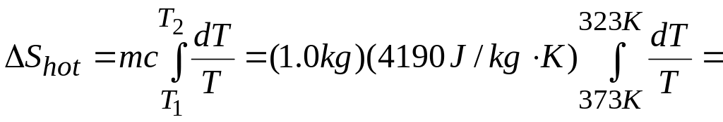
J/K.

The entropy change of the cold water is

J/K.

The total entropy change of the system is

= (-603 J/K) + 705 J/K = +102 J/K

EVALUATE: An irreversible heat flow in an isolated system is accompanied by an increase in entropy. We could have reached the same end state by simply mixing the two quantities of water. This, too, is an irreversible process; because the entropy depends only on the state of the system, the total entropy change would be the same, 102 J/K.

It's worth noting that the entropy of the system increases continuously as the two quantities of water come to equilibrium. For example, the first 4190 J of heat transferred cools the hot water to 99°C and warms the cold water to 1°C. The net change in entropy for this step is approximately

J/K

Can you show in a similar way that the net entropy change is positive for any one-degree temperature change leading to the equilibrium condition?

Entropy and the Second Law

The results of Example 20.10 about the flow of heat from a higher to a lower temperature, or the mixing of substances at different temperatures, are characteristic of all natural (that is, irreversible) processes. When we include the entropy changes of all the systems taking part in the process, the increases in entropy are always greater than the decreases. In the special case of a reversible process, the increases and decreases are equal. Hence we can state the general principle:

When all systems taking part in a process are included, the entropy either remains constant or increases.

In other words: No process is possible in which the total entropy decreases, when all systems taking part in the process are included.

This is an alternative statement of the second law of thermodynamics in terms of entropy. Thus it is equivalent to the "engine" and "refrigerator" statements discussed earlier.

The increase of entropy in every natural, irreversible process measures the increase of disorder or randomness in the universe associated with that process. Consider again the example of mixing hot and cold water (Example 20.10). We might have used the hot and cold water as the high- and low-temperature reservoirs of a heat engine. While removing heat from the hot water and giving heat to the cold water, we could have obtained some mechanical work. But once the hot and cold water have been mixed and have come to a uniform temperature, this opportunity to convert heat to mechanical work is lost irretrievably. The ukewarm water will never unmix itself and separate into hotter and colder portions. No decrease in energy occurs when the hot and cold water are mixed. What has been lost is not energy, but opportunity, the opportunity to convert part of the heat from the hot water into mechanical work. Hence when entropy increases, energy becomes less available, and the universe becomes more random or "run down."

20.8 Microscopic Interpretation of Entropy

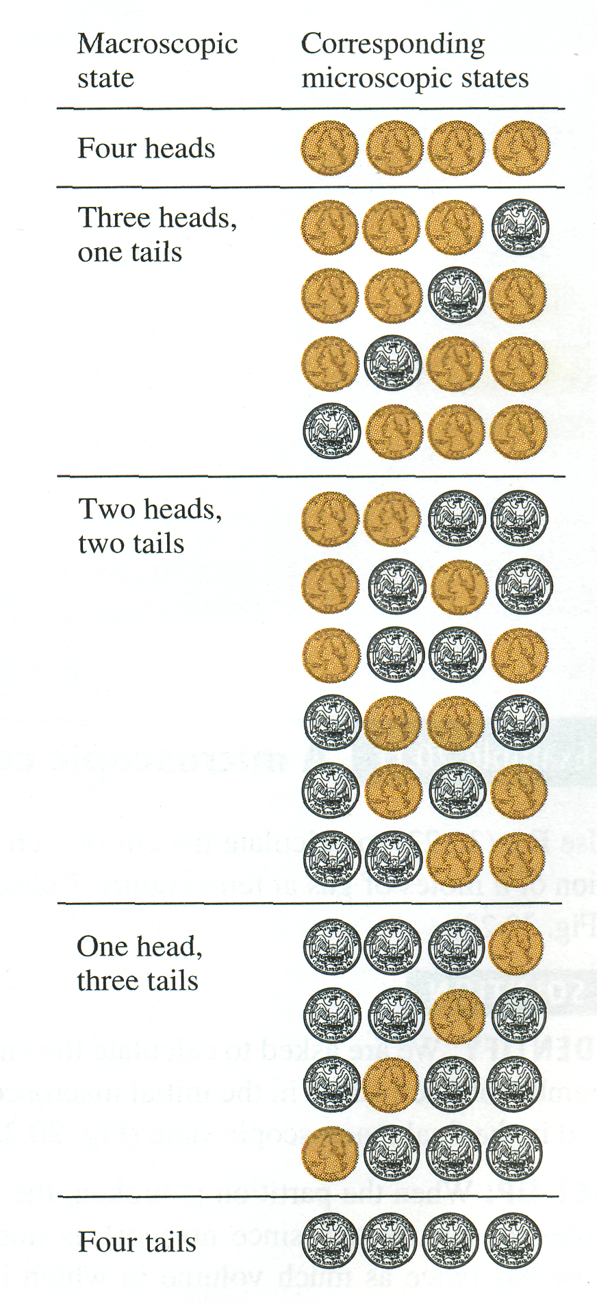
We described in Section 19.4 how the internal energy of a system could be calculated, at least in principle, by adding up all the kinetic energies of its constituent particles and all the potential energies of interaction among the particles. This is called a microscopic calculation of the internal energy. We can also make a microscopic calculation of the entropy S of a system. Unlike energy, however, entropy is not something that belongs to each individual particle or pair of particles in the system. Rather, entropy is a measure of the disorder of the system as a whole. To see how to calculate entropy microscopically, we first have to introduce the idea of macroscopic and microscopic states.

Suppose you toss N identical coins on the floor, and half of them show heads and half show tails. This is a description of the large-scale or macroscopic state of the system of N coins. A description of the microscopic state of the system includes information about each individual coin: Coin 1 was heads, coin 2 was tails, coin 3 was tails, and so on. There can be many microscopic states that correspond to the same macroscopic description. For instance, with N = 4 coins there are six possible states in which half are heads and half are tails (Fig. 20.22). The number of microscopic states grows rapidly with increasing N; for N = 100 there are 2¹⁰⁰ = 1.27 X 10³⁰ microscopic states, of which 1.01 X 10²⁹ are half heads and half tails.

The least probable outcomes of the coin toss are the states that are either all heads or all tails. It is certainly possible that you could throw 100 heads in a row, but don't bet on it; the probability of doing this is only 1 in 1.27 X 10³⁰. The most probable outcome of tossing N coins is that half are heads and half are tails. The reason is that this macroscopic state has the greatest number of corresponding microscopic states, as shown in Fig. 20.22.

To make the connection to the concept of entropy, note that N coins that are all heads constitute a completely ordered macroscopic state; the description "all heads" completely specifies the state of each one of the N coins. The same is true if the coins are all tails. But the macroscopic description "half heads, half tails" by itself tells you very little about the state (heads or tails) of each individual coin. We say that the system is disordered because we know so little about its microscopic state. Compared to the state "all heads" or "all tails," the state "half heads, half tails" has a much greater number of possible microscopic states, much greater disorder, and hence much greater entropy (which is a quantitative measure of disorder).

Now instead of N coins, consider a mole of an ideal gas containing Avo-gadro's number of molecules. The macroscopic state of this gas is given by its pressure p, volume V, and temperature T; a description of the microscopic state involves stating the position and velocity for each molecule in the gas. At a given pressure, volume, and temperature, the gas may be in any one of an astronomically large number of microscopic states, depending on the positions and velocities of its 6.02 X 10²³ molecules. If the gas undergoes a free expansion into a greater volume, the range of possible positions increases, as does the number of possible microscopic states. The system becomes more disordered, and the entropy increases as calculated in Example 20.8 (Section 20.7).

We can draw the following general conclusion: For any system, the most probable macroscopic state is the one with the greatest number of corresponding microscopic states, which is also the macroscopic state with the greatest disorder and the greatest entropy.