Inventory system with a fixed periodicity of purchase orders

The orders to be performed consequently after the fixed time periods (week, month, etc). Inventory level to be checked at the end of each interval; then delivery volume depends on consumption history.

The inventory volume can be changed by shifting a lot (order) size.

The volume of purchase order is subject to change; depends on resources consumption during the preceding period.

P.O. size = Maximum fixed inventory level – actual inventory volume at the period of an order.

Parameters: Max. inventory level; and fixed time lag (interval between two orders).

Disadv: after expiration of a “period” the small order might be taken; or can be a deficit, if consumption increases before its time to prepare a new order.

Cases when used:

Costs of preparing orders and deliveries are relatively low; losses as a deficit consequence are not high; the purchase volumes can be managed.

System “Minimum-maximum”

The fixed interval between orders being used. System might be implemented when accounting inventory costs and preparing purchase orders happen to be very high, and can be compared to the losses if inventory deficit.

Two inventory levels are settled – min. and max. When inventory drops till or below “min.”, a new order to be taken, up till the “max” level.

System with a preset sequence of orders to replenish inventory levels till the specified volume (система с установленным периодом пополнения запасов до заданного уровня).

When: high demand fluctuations.

To prevent over-stocks or a deficit, the orders prepared not only periodically, but upon achieving the critical inventory levels. The system combines elements of “fixed periodicity” and “critical point of purchase order”.

P. Orders: “planned” and “additional”. If inventory drops lower “min. point of p.o.” – the additional (extraordinary) p.o. to be performed. In other times – works as a system with a fixed orders periodicity.

P.O. size – forecasting inventory consumption till the new order will be delivered to a storehouse.

System of “operating management”(ukr): after certain time lags the decisions to be taken: to order or not, and which quantities.

4. ABC-XYZ analysis

At the basis – “Pareto” rule – 80/20. The major part of inventory costs corresponds to their relatively small quantity.

ABC analysis – to discover the distribution degree of a certain characteristic between the elements of a variety (множество).

The elements to be distributed into three (A,B,C) parts, according to their comparative impact on the total inventory costs.

Algorithm:

1. Define value of each commodity (using purchasing prices)

2. Place commodities upon price decrease

3. Summarize quantities and costs of purchase;

4. Grouping according to their relative value in general purchasing costs.

A group: the most expensive goods with 70-80% inventory value, but their quantity amounts 10-

20% of general inventory number;

B – average valued costs; value – 10-15%, quantity – 30-40%;

C – the cheapest; 5-10% of general value, but 40-50% of the general quantity.

ABC analysis permits classification of product assortment according to their value.

XYZ analysis

Product assortment to be differentiated according to demand fluctuations and forecast accuracy.

X group – uniform (рівномірний) demand; easy to forecast sales

Y – fluctuating demand; seasonal nature. Average forecasting possibilities.

Z – episodic demand, absence of tendencies; difficult to forecast.

To put into the certain group (x,y,z) the demand variation coefficient being used:

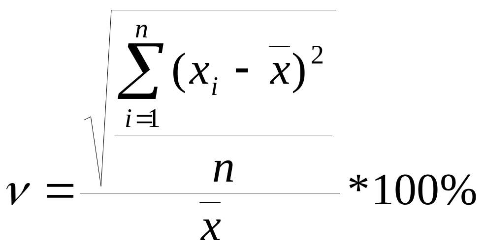
- coefficient of demand variation;

- i- demand value for a certain product (i - значение спроса по оцениваемой позиции )

- average demand value for the position under question, period n (среднее значение спроса по оцениваемой позиции, за период n)

- period lag the evaluation being performed for (размер периода по которому делалась оценка)

Variation coefficient can change from 0 till (infinity). Breaking into groups – algorithm (table 1):

Group	Interval
X	0 υ<10%
Y	10% υ<25%
Z	25% υ<

The general algorithm:

• Defining coefficients of variations for the different assortment positions;

• Grouping managing objects according to variation coefficient increase; creating a table with

corresponding coefficients;

• Designing XYZ graph;

• Distribution managerial object into three groups: X, Y, Z (table 1)

• Creation a matrix ABC-XYZ, highlighting positions where a particular control needed (final).

	A group	B group	C group
X- material	High consumer value	Average consumer value	Low consumer value
	High forecast effect	High forecast effect	High forecast effect
Y- material	High consumer value	Average consumer value	Low consumer value
	Average forecast effect	Average forecast effect	Average forecast effect
Z- material	High consumer value	Average consumer value	Low consumer value
	Low forecast effect	Low forecast effect	Low forecast effect

The matrix provides useful tools for planning and management both for purchasing logistics and inventory logistics.

XYZ graph

К оефіцієнт

в аріації попиту 100

%

1 00

Позиції асортименту, що побудовані у порядку зменшення долі у загальному запасі, у процентах до загальної кількості позицій, %

Assortment position built according to decreasing of their value (%) to the general quantity of positions, %

1 Douglas M.Lambert and James R. Stock, Strategic Logistic Management, 3^rd ed. – Homewood IL: R. D. Irwin, 1993. – p. 368