Invitation to a Contemporary Physics (2004)

give a flavor of things, we write down the equations obeyed by these variables:

X˙ = σ(Y − X)

Y˙ = γX − Y − XZ

Z˙ = XY − bZ .

These are the equations that Lorenz studied in 1963 as his model for weather. The overhead dot denotes the rate of change with time. Here, σ (sigma), γ (gamma) and b are parameters defining the conditions of the experimeter. Thus, b is a geometry factor (depending on a certain aspect ratio). Sigma (called the Prandtl number) measures the ratio of viscosity to thermal conductivity-times-density, and

γis the control parameter — the Rayleigh number normalized in a certain way. In our experiment, as you increase the temperature di erence from zero, you increase

γfrom zero. For γ between zero and one, we have the steady di usion of heat. For γ greater than 1 but less than about 24.74, steady convective rolls develop. Eventually, for γ greater than about 24.74 we have motion on a strange attractor giving chaos (the Lorenz attractor).

A strange attractor in three dimensions is hard to visualize. One could either resort to making Poincar´e sections, or just look at the projection on a plane (see Fig. 7.10).

One can readily see that the trajectory winds around an unstable fixed point

C, spirals outward and after reaching out to a critical distance from C, crosses over to wind around the other unstable fixed point C . The number of circuits

the trajectory makes around any one of the unstable fixed points before it switches to the other, generates a sequence which is as random as the tossing of a fair coin.

Z

Y

Figure 7.10: The Lorenz (strange) attractor projected on Y Z-plane. C and C are two unstable fixed points. The strange attractor depicts chaos (schematic).

It turns out that the trajectories are actually confined to a sheet of small but finite thickness, within which is embedded the entire complex geometry of the attractor; it is a fractal.

The Lorenz system turns out to describe other systems as well, for example the irregular spiking of laser outputs. The irregular reversal of Earths’ magnetic field, in the geodynamo dynamo model, may be linked to the random jumping of the trajectory between C and C .

7.4.7Routes to Chaos

We have seen that chaos is described by strange attractors. In most of the physically interesting cases these attractors are the low-dimensional ones. We will now summarize two commonly observed routes to chaos described by such low-dimensional strange attractors.

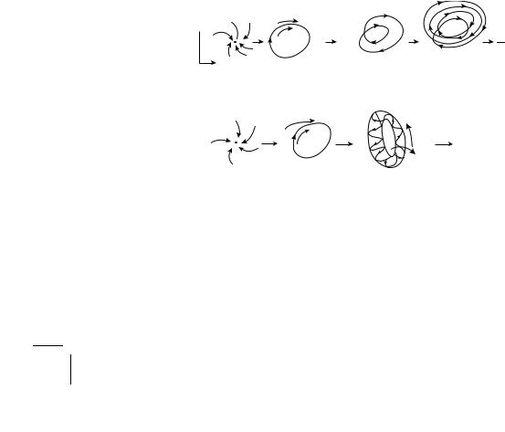
The first route is that of an infinite sequence of period-doubling bifurcations as the control parameter is varied. We begin with a stable fixed point (stationary point) that becomes unstable and bifurcates to a limit cycle (aperiodic orbit), which undergoes a period-doubling sequence leading to a pile-up, that is, an accumulation point (periodic orbit) — the onset of chaos. This is the Feigenbaum scenario that we have already come across in the case of the leaky faucet. It is also the route followed by convective turbulence (Lorenz attractor). This route has already been shown schematically as the bifurcation plot for the logistic map. In Fig. 7.11a we show this route in terms of the projection of the phase trajectory in a plane.

There is another route to chaos that is qualitatively di erent. Here, we start with a stable fixed point (stationary point) that becomes unstable and bifurcates to

Y

Figure 7.11: Routes to chaos involving (a) an infinite number of period-doubling bifurcations;

(b) a finite number of topological transitions.

a limit cycle (a periodic orbit). The limit cycle in turn becomes unstable and bifurcates to a biperiodic torus (doubly periodic orbit) with incommensurate frequencies, i.e., quasiperiodic. Finally, from the biperiodic torus we jump to chaos — without any intervening sequence of appearances of new frequencies. This is the sequence leading to turbulence observed in the Couette flow discussed earlier. Here, the fluid is confined to the annular space between two coaxial cylinders, one of which is made to spin. In Fig. 7.11b we have shown schematically this route to chaos.

It is important to appreciate a qualitative di erence between these two routes to chaos. In the first route (period-doubling route), it is simply the period of the limit cycle that changes at bifurcation. No new states are being generated. In the second route, the bifurcation from the limit cycle to the torus is a topological change involving new states.

There are other routes to chaos possible. But there is no experimental evidence for the Landau scenario involving the appearance of incommensurate frequencies, one at a time, leading eventually to a confusion that we would call chaos.

7.5 Fractals and Strange Attractors

Fractals are geometrical objects with shapes that are irregular on all length scales no matter how small: they are self-similar, made of smaller copies of themselves. To understand them, let us re-examine some familiar geometrical notions.

We know from experience that our familiar space is three-dimensional. That is to say that we need to specify three numbers to locate a point in it. These could, for example, be the latitude, the longitude and the altitude of the point giving respectively, its north-south, east-west, and the up-down positions. We could, of course, employ a Cartesian coordinate system and locate the point by the triple (x, y, z). Any other system of coordinates will equally su ce. The essential point is that we need three numbers — more will be redundant and fewer won’t do. Similarly, a surface is two-dimensional, a line one-dimensional and a point has the dimension of zero.

These less-dimensional spaces, like the two-dimensional surface, the onedimensional line, or the zero-dimensional point, may be viewed conveniently as embedded in our higher three-dimensional space. All these ideas are well known from the time of Euclid and underlie our geometrical reckoning. So intimate is this idea of dimension that we tend to forget that it has an empirical basis. Thus, it seems obvious that the dimension has to be a whole number. Indeed, the way we have defined the dimension above it will be so. (We call it the topological dimension, based on the elementary idea of neighborhood.) There is, however, another aspect of dimensionality that measures the spatial content or the capacity. We can ask, for instance, how much space does a given geometrical object occupy. Thus, we speak of the volume of a three-dimensional object. It scales as the cube of its linear size —

if the object is stretched out in all directions by a factor of 2, say, the volume will become 23 = 8 times. Hence, it is three-dimensional. Similarly, we speak of the area of a surface that scales as the square of its linear size, and the length of a line that scales as the first power of the linear size. As for the point, its content, whatever it may be, stays constant — it scales as the zeroth power of the linear size, we may say. In all these cases, the ‘capacity dimension’ is again an integer and agrees with the topological dimension.

But this need not always be the case. To see this, let us consider the measurement operation in some detail. Consider a segment of a straight line first. To measure its length we can use a divider as any geometer or surveyor would. The divider can be opened out so that the two pointed ends of it are some convenient distance apart. This becomes our scale of length. Let us denote it by L. Now all that we have to do is to walk along the line with the divider marking o equal divisions of size L. Let N(L) be the number of steps (divisions) required to cover the entire length of the line. (There will be some rounding o error at the end point which can be neglected if it is su ciently small so that N(L) 1.) Then the length of the segment is L = LN(L). Let us now repeat the entire operation but with L replaced by L/2, that is, with the distance between the divider end points halved. The number of steps will now be denoted by N(L/2). Now we must have L = LN(L) = (L/2)N(L/2). This is because we have covered exactly the same set of points along the straight line skipping nothing and adding nothing. Thus, halving the measuring step length simply doubles the number of steps required. This can be restated generally as the proportionality or scaling relation N(L) L−1, that is, the number of steps N(L) required is inversely proportional to the size L of the linear step length for small enough L. This seems obvious enough. The ‘1’ occuring in the exponent gives the capacity dimension (D) of the straight line. In a more sophisticated language, D = −(d ln N(L)/d ln L) as L → 0. In our example this indeed gives D = 1. Here, ln stands for the natural logarithm. Thus, finding the capacity dimension is reduced to mere counting. It is indeed sometimes referred to as the box counting dimension.

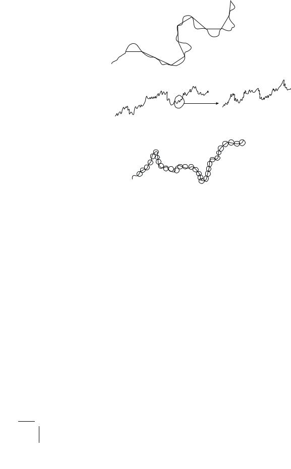
So far so good. But what if we have a curved line? For, in this case as we walk along the line with our divider, we will be measuring the chord length of the polygon rather than the true arc length of the curved line, as can readily be seen from Fig. 7.12a.

Are we not cutting corners here? Well, no. The point is this. If the curve is a smooth one, it will be straight locally. Thus, as we make our step length L smaller and smaller, the chords will tend towards the arcs, and the polygon will approximate the curve better and better, until it eventually hugs the curve as L → 0. (This is the significance of the proviso L → 0 in our logarithmic formula.) In the end, therefore, there is no distinction between the case of the straight line and that of a curved but smooth line: in both the cases, we will get D = 1. The smooth curve is rectifiable! Thus, all smooth curves have the same capacity dimension D = 1.

ε

(a)

Magnification

(b)

ε

(c)

Figure 7.12: (a) Covering a line with scale length ; (b) self-similarity of a fractal curve;

(c) covering a line with discs or balls.

Curves that are smooth, that is, straight locally (viz., have a well-defined tangent) are said to be regular. Now, what if the curve is irregular — that is to say, if it has a zig-zag structure down to the smallest length scale? You take a small segment of it that looks smooth enough at the low resolution of the naked eye and then view it again under a magnifying lens of higher resolution. It may reveal an irregularity that looks just the same as that of the original curve. We say that the irregularity is self-similar (Fig. 7.12b). It has no characteristic length scale below which it is smooth. It is like the infinite ‘matryoshka’ with a doll within a doll within a doll, ad infinitum, all exactly alike but for the size. How do you find the dimension and the length of such an irregular curve? Intuition is no guide now. But we can get back to our divider and walk the curve as before. The polygon traversed by us will now never quite hug the irregular curve. But we still have our L and N(L), and we can hopefully find the scaling N(L) L−D as L → 0. The exponent D is then the capacity dimension of the curve by our definition. However, D is now not necessarily an integer. It will, in general, be a fraction! The zig-zag curve is then called a fractal and D its fractal dimension. For example, we may survey the irregular coastline of England and find that it is a fractal, with a fractal dimension

260 Chaos: Chance Out of Necessity

of about 1.3. What about the length of this fractal coast line? Well, we still have L LN(L). Thus, as L → 0, the length of the coastline tends to infinity! The length depends on the scale of resolution. It was the study of such irregular shapes and forms that had led Benoit Mandelbrot of IBM to the discovery of fractals and fractal geometry in 1960.

A fractal line is something intermediate between a one-dimensional line and a two-dimensional surface. The fractal line with its self-similar irregularity structure down to the finest length scale has an amusing but revealing aspect to it. If we were to run the needle of a gramophone on such a fractal track (groove), it will produce a symphony that is independent of the speed of the needle! The scale invariance in space gets translated into a scale invariance in time via the constant speed of traversal of the groove by the needle.

The same ideas can now be extended to an irregular (fractal) surface. In this case, of course, we will employ elementary squares or plaquettes measuring L on the side, to cover the surface. If N(L) is the number of plaquettes required to cover it, then we expect N(L) L−D, where D is the fractal dimension. In all these examples, our geometrical objects, the lines (topological dimension 1) and the surfaces (topological dimension 2), are assumed to be embedded in the background Euclidean space of topological dimension 3, which is our familiar space. But we can always imagine our objects to be embedded in a background Euclidean space of a higher dimension denoted by d. We will call this the embedding dimension. It is important to realize that the fractal dimension of the geometrical object is its intrinsic property. It does not depend on the space in which it may happen to be embedded. Of course, the embedding space must have a Euclidean dimension greater than the topological dimension of the object embedded in it. Thus, for example, a zig-zag curve embedded in our three-dimensional Euclidean space may be ‘covered’ with three-dimensional L-balls or L-boxes instead of one-dimensional L- segments (Fig. 7.12c). The intrinsic fractal dimension will work out to be the same, and it shall be greater than unity, even up to infinity. Such an intrinsic fractal dimension is relevant for reckoning the weight of an irregular (zig-zag) thread, a linear polymer such as a highly random coiled DNA strand, say. We could also define an extrinsic fractal dimension for the irregular line — it now measures the basin wetted by the line. But, this extrinsic fractal dimension can at most be equal to the embedding dimension — here the line fills the space!

And now we are ready for an important generalization. We will ask for the fractal dimension of a set of points embedded in a Euclidean space of dimension d. We need this generalization for our study of chaos. Because here the background Euclidean space is the state space that can have any integral dimension. In this state space the set of points, or more like a dust of points is embedded forming the attractor whose fractal dimension (D) we are after. The dimension d of the state space is the embedding dimension. Our method remains the same. We cover the set of points with d-dimensional balls of radius L and then fit the scaling relation

N(L) L−D or use the equivalent logarithmic formula discussed earlier. All this can be done rather quickly on a PC. It is, however, important to appreciate that the scaling relation, e.g., N(L) L−1, ceases to have any physical validity in the limit when L becomes comparable with the microscopic size of the atoms or the size of the macroscopic object. The scaling holds only in the interesting region of intermediate asymptotics. The whole point is that this intermediate scaling region covers a su ciently wide range 102–104. Hence the operational validity of the notion of the fractal. Of course, mathematicians have constructed a few truly fractal curves. But nature abounds in physically fractal objects — e.g., lightening discharges, cloud contours, coastlines, mountain ranges, fractures, crumpled paper balls, di usion-limited aggregates (spongy masses), biological sponges, foams, human and animal lungs, human cortex foldings, protein surface folds. The clustering of galaxies suggests a large scale mass structure of the universe with a fractal dimensionality D 2, that may account for the missing mass that astronomers and cosmologists are very much concerned with. As to why Nature abounds in fractals, the answer may lie in what is known as self-organized criticality (SOC). Forms in Nature often emerge from recursive growth building up to the point of instability and breakdown, giving a landscape which is rough on all length scales — a critical state, a self-similar fractal!

Before we go on to the fractal attractors, let us get acquainted with some of the fascinating fractals that have become classics. We will actually construct them.

7.5.1 The Koch Snowflake

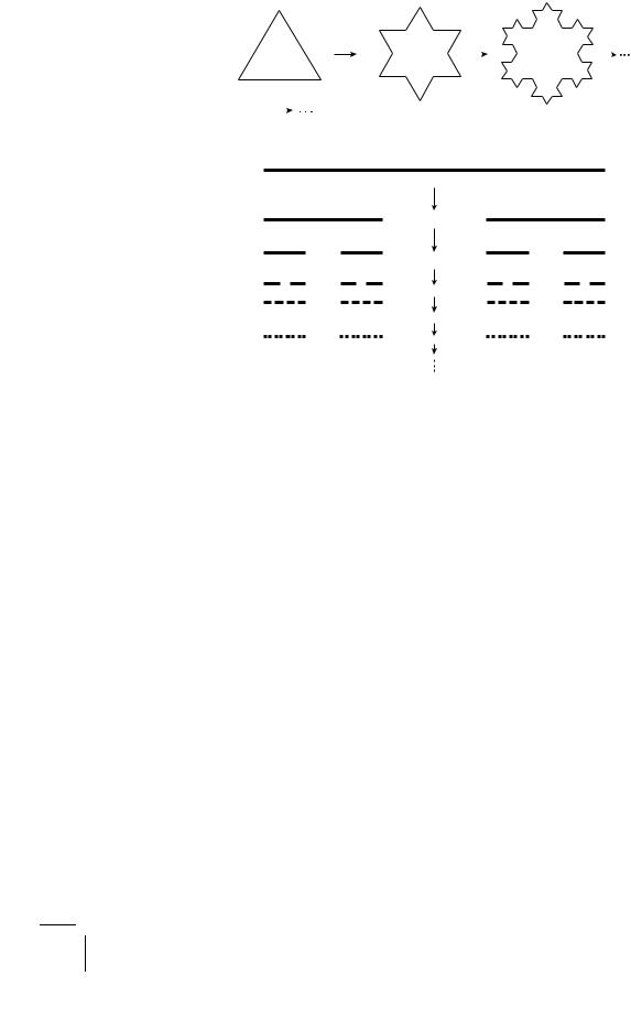
Take an equilateral triangle. Now divide each side in three equal segments and erect an equilateral triangle on the middle third. We get a 12 sided Star of David. The construction is to be iterated ad infinitum. Smaller and smaller triangles keep sprouting on the sides and finally we have a zig-zag contour that is irregular on all length scales in a self-similar fashion, resembling a snowflake (Fig. 7.13).

To find its fractal dimension, all we have to note is that at each iteration the scale of length gets divided by 3 and the number of steps required to cover the perimeter increases by a factor of 4. This gives the fractal dimension D = − ln 4/ ln(1/3) = 1.26. It is interesting to note that while the actual length of the perimeter scales as (4/3)n to infinity as expected, the area enclosed by the figure remains finite, close to that of the original triangle.

7.5.2 Cantor Dust

Take a segment of a straight line of unit length, say. Trisect it in three equal segments and omit the middle third, retaining the two outer segments (along with their end points). Now iterate this construction by trisecting these two segments and again omitting the middle thirds, and so on ad infinitum. Eventually, you would

Figure 7.13: Koch snowflake. Construction algorithm for this fractal of dimension 1.26.

Figure 7.14: Cantor dust. Construction algorithm for this fractal of dimension 0.63.

be left with a sparse dust, called the Cantor set, of uncountably infinite points (Fig. 7.14). What is its capacity dimension? Well, in each iteration, the length of the segments gets divided by 3 while the number of such segments is multiplied by 2. Hence the fractal dimension D = − ln 2/ ln(1/3) = 0.630. Of course the total length of the set at the nth iteration is (2/3)n, which tends to zero as n → ∞.

Aside from these and many other fascinating examples of fractal sets, which are just mathematical constructs, we do have fractal objects occurring in Nature. We have already mentioned several of them occurring naturally. Indeed, a fractal geometry should be Nature’s strategy for enhancing the surface to volume ratio.

The fractal dimension D is a purely geometrical measure of the capacity of a set. Thus in ‘box counting,’ all the boxes, or rather the neighborhoods, are weighted equally. In the context of chaos, however, a fractal is a set of points in the state space on which the ‘strange attractor’ lives. The di erent neighborhoods (boxes) of the fractal are visited by the phase point with di erent frequency in the course of its ‘strange’ aperiodic motion; the fractal set is physically inhomogeneous. The fractal dimension D as defined above fails to capture this physical fact. It is possible to define yet another fractal dimension that weights di erent neighborhoods according as how frequently they are visited. In fact a whole spectrum of fractal dimensions are defined in what is called multifractal analysis of the fractal set. This is a highly technical matter and we will not pursue it further here. Su ce to say that

the multifractal analysis combines geometry with physics and thus reveals more information.

7.6Reconstruction of the Strange Attractor from a Measured Signal: The Inverse Problem

A dynamical system may have a number of degrees of freedom. This whole number is the dimension ‘d’ of its phase space. The dynamics will eventually settle down on an attractor. If the dynamics is chaotic, it will be a strange attractor (a fractal) of fractional dimension D, imbedded in the phase space of (imbedding) dimension d > D. Both d and D are important specifications of the nature of the system and its strange attractor. Now, in general, these two dimensions are not given to us. All we have is an experimentally observed, seemingly random signal representing the measurement of a single component of the d-dimensional state vector in continuous time. It could, for instance, be the temperature in a convection cell, or a component of fluid velocity of a turbulent flow at a chosen point. This can be measured, for example, by the Laser Doppler Interferometry, in which the frequency of a laser light scattered by the moving liquid at a point is Doppler shifted. The shift is proportional to the instantaneous velocity of the fluid at that point. The question is, can we reconstruct these important attributes such as D and d from such a single-component measurement in time? It was proved by Floris Takens that we can indeed retrieve some such vital information about the system from this stream of single-component data.

The philosophy underlying this claim is quite simple. In a dynamical system with interacting degrees of freedom, where everything a ects everything all the time, it is conceivable, indeed highly plausible, that a measurement on any one of them should bear the marks of all others, however implicitly. The real question now is how to recover this information. This is a rather technical matter. The technique is, however, very straightforward to apply and is worth knowing about.

Let us take x(t) to be the measured signal. The first step is to discretize time. For this, pick a convenient time interval τ and form the sequence x(t), x(t + τ), x(t + 2τ), . . . . This is known as a time series. Next, we are going to construct vectors out of this series. First, construct the two-dimensional vectors (x(t), x(t + τ)), (x(t + τ), x(t + 2τ)), (x(t + 2τ), x(t + 3τ)), . . . . Each vector has two Cartesian components, for example x(t) and x(t + τ), as any two-dimensional vector should. Plot these vectors in a two-dimensional phase space, so as to generate a dust of points. Now, count how many neighbors a point has, on average, lying within a radius of it. Let the number be C(L). For small L, we will find that C(L) scales as C(L) Lν. Then, ν is said to be the correlation dimension of our set. We will use a subscript and call it ν2 because we constructed it from a two-dimensional phase space. Now repeat this procedure, but this time with the three-dimensional vectors constructed

out of our time-series, i.e., (x(t), x(t+τ), x(t+2τ)), (x(t+τ), x(t+2τ), x(t+3τ)), . . . .

Each vector has three Cartesian components. We will, therefore, get the correlationdimension ν3 this time. And so on. Thus, we generate the numbers ν1, ν2, ν3, . . . .

We find that νn will saturate at a limiting value, a fraction generally, as n becomes su ciently large. That limiting value is then the Correlation Dimension of the Attractor of our system. It is usually denoted by D2 and is less than or equal to the fractal dimension D of the attractor. Also, the value of the integer n, beyond which νn levels o , is the minimum imbedding dimension of our attractor. That is, it is the minimum number of degrees of freedom our dynamical system must have to contain this attractor.

This technique, due to P. Grassberger and I. Procaccia, seems to work well with low dimensional attractors. It has been used extensively to characterize chaos in all sorts of systems including the human cortex. Thus, the EEG time series for various brain-wave rhythms, e.g., with eyes closed, with eyes open, with and without epileptic seizure have been analyzed with startling results. The epileptic brain is less chaotic (i.e., it has lower fractal dimension) than the normally active brain!

The time-series analysis and reconstruction of the attractor provides other important information as well. It can distinguish deterministic chaos from truly random noise. Thus, for example, the correlation dimension D2 is infinite for random noise, but finite and greater than two for chaos. (For a limit cycle, it is one and for a torus (quasiperiodic) it is two). Thus, we know, for example, that the noisy intensity output of a laser can be due to a low dimensional strange attractor in its dynamics.

7.7 Concluding Remarks: Harvesting Chaos

That a simple looking dynamical system having a small number of degrees of freedom and obeying deterministic laws can show chaos is a surprise of classical physics. It has made chaos a paradigm of complexity — one that comes not from the statistical law of large numbers, but from the highly fine-structured self-similar organization in time and space. There is no randomness put in by hand. Chaos is due to the sensitive dependence on initial conditions that comes from the stretching and folding of orbits. Mathematically, this is represented by the all important nonlinear feedback. Thus, chaos can amplify noise, but it can also masquerade as ‘noise’ all by itself. It is robust and occurs widely. It has classes of universality.

The theory of chaos rests on a highly developed mathematical infra-structure that goes by the forbidding name of nonlinear dynamical systems. But high-speed computing has brought it to within the capability of a high school student. The contemporaneous ideas of fractal geometry have provided the right language and concepts to describe chaos.