

366 |
Broadband Microstrip Antennas |
within the BW for VSWR = 2 of the SM antenna. In the E-plane, the radiation pattern of the SM is similar to that of the thin monopole antenna. With an increase in frequency from 1.5 GHz to 2.5 GHz, the variation in the azimuthal pattern (H-plane) increases from 1 dB to 3 dB for SM, because of the asymmetry in the X- and Y-planes of the structure as compared to the thin monopole antenna.
9.2.5 Various Planar RMs with Equal Areas
After observing the effects of various parameters on the BW of the monopole antenna, the dimensions L and W of RM are chosen such that their surface areas are equal, so that a comparison of performances of these planar monopole antennas may be made. For all the measurements, the size of the ground plane is chosen to be 30 cm × 30 cm with p = 0.1 cm. The SM is fed in the middle of the one side by a SMA connector as shown in Figure 9.6(a), whereas RM is fed in two different ways as shown in Figure 9.6(b, c). The RMs with feeds in the middle of the smaller and larger dimensions are coined RMAs and RMBs, respectively.
The dimensions and VSWR BW of these configurations are listed in Table 9.2. The theoretical lower frequency f L for VSWR = 2 obtained using (9.8), is also tabulated. The percentage error is calculated using
%error = |
f L − f m |
× 100 |
(9.9) |
|
f m |
||||
|
|
|
where f m is the lower measured frequency. The theoretical frequencies predicted by (9.8) are within ±6.6% of the measured values. The f L of RMB
Figure 9.6 (a) Square monopole antenna. RM antennas with feed in the middle of (b) smaller W and (c) larger W.
Broadband Planar Monopole Antennas |
367 |
Table 9.2
Comparison of Square, Rectangular, Triangular, and Hexagonal Monopole Antennas
|
|
|
Measured |
|
|
|
|
|
|
|
Frequency f m |
|
|
|
|
|
|
|
Range for |
|
|
Percentage |
|
|
L × W |
VSWR ≤ 2 |
|
Measured |
Error in |
||
Configuration |
(cm × cm) |
(GHz) |
f L (GHz) |
BW Ratio |
Frequency |
||
SM |
4.5 |
× 4.5 |
1.27 |
to 2.81 |
1.354 |
1:2.2 |
+6.6 |
RMA |
4.6 |
× 4.2 |
1.38 |
to 2.75 |
1.341 |
1:2.0 |
−2.8 |
RMB |
4.2 |
× 4.6 |
1.40 |
to 2.02 |
1.431 |
1:1.4 |
+2.2 |
TMB |
5.9 |
× 6.8 |
1.07 |
to 1.11 |
1.101 |
1:1.04 |
+2.9 |
HMA |
4.8 |
× 5.6 |
1.37 |
to 2.68 |
1.282 |
1:1.9 |
−6.5 |
HMB |
5.6 |
× 4.8 |
1.20 |
to 3.92 |
1.147 |
1:3.2 |
−4.4 |
|
|
|
|
|
|
|
|
is higher than that of the RMA, because the height of the RMB is smaller than that of the RMA.
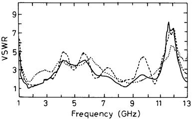
The measured VSWR plots of SM, RMA, and RMB are given in Figure 9.7. The VSWR values fluctuate from as high as 8 to as low as 1.05 in the frequency range of 1–13 GHz. The measured BW ratios of SM, RMA, and RMB in the lower range of frequency are 1:2.2, 1:2.0, and 1:1.4, respectively. By adjusting the dimensions of the patches and length of the
Figure 9.7 Measured VSWR plots for three monopole antennas: ( —— ) SM, ( - - - ) RMA, and ( ? ? ? ) RMB.
368 |
Broadband Microstrip Antennas |
probe, these configurations can be optimized to operate within selected frequency bands.
9.3 Planar Triangular and Hexagonal Monopole Antennas
Other polygon variations of planar monopole antennas, such as triangular and hexagonal monopole (TM and HM) antennas, are considered next. The surface area and other parameters of these monopoles are kept the same as those of the rectangular and square monopoles for comparison.
9.3.1 Planar Equilateral Triangular Monopole
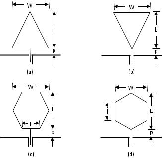
The side length of the equilateral triangular patch is calculated to be 6.84 cm, so that its area is equal to that of the SM described in the previous section. Two feed configurations, TMA and TMB, are considered as shown in Figure 9.8(a, b). The TMA is fed at the middle of the side while the
Figure 9.8 Triangular monopole antenna fed (a) in the middle of the side and (b) at the vertex. Hexagonal monopole antenna fed (c) in the middle of the side and (d) at the vertex.
Broadband Planar Monopole Antennas |
369 |
TMB is fed at the vertex. The TMB configuration is equivalent to one-half of broadband bowtie dipole antenna [5].
For calculating f L of the TMA and TMB antenna using (9.8), the values of L and r of the effective cylindrical monopole are determined as
L = √ |
3W /2 |
|
(9.10) |
r = W /(4p) |
(9.11) |
||
where W is equal to the side length of the equilateral triangle.
For TMA, the VSWR is always greater than 2, as there is no input impedance matching at any frequency. However, for TMB, which is like a half-bowtie dipole, matching is obtained at some frequencies. The results for the TMB are summarized in Table 9.2. The f L of this antenna is the least amongst all the other configurations of the same area because it has the largest height. The measured BW is smaller as compared to the corresponding RM and SM antennas.
9.3.2 Planar Hexagonal Monopole
The side length l of the hexagon is obtained by equating its area with SM, and its value is calculated to be 2.8 cm. In this case also, two feed configurations, HMA and HMB, are used as shown in Figure 9.8(c, d). The HMA and HMB are fed in the middle of the side and at the vertex, respectively. The theoretical lower frequencies corresponding to VSWR = 2 are calculated separately for the HMA and HMB antennas as given below.
For the HMA, the L and r values of the equivalent cylindrical monopole antenna are obtained by equating their areas as follows:
L |
= √ |
3l |
|
(9.12) |
||
r = |
3l /(4p ) |
(9.13) |
||||
The parameters for the HMB are: |
|
|||||
L = 2l |
(9.14) |
|||||
r = 3√ |
|
l /(8p ) |
|
|||
3 |
(9.15) |
|||||
370 |
Broadband Microstrip Antennas |
For these values of L and r, the lower frequency f L is computed from
(9.8).
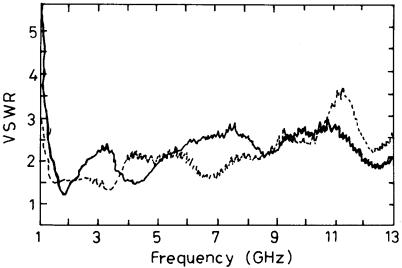
The VSWR plots for these two configurations are shown in Figure 9.9, and the results are summarized in Table 9.2. The f L of HMB is lower than that of HMA because of its larger height L . The HMB has a larger BW than the HMA. This can be understood from the analogy that the HMB feed is similar to that of the TMB, which yields better matching than the TMA. The HMA feed is similar to the feed for the TMA and hence yields a smaller BW. The HMB provides a wider BW than the square and the RMs, as it is closer to the circular configuration, which has a very large BW as described in the next section.
9.4 Planar Circular Monopole Antennas
A planar circular monopole (CM) antenna yields very broad BW [1, 2]. A CM of radius a is shown as inset in Figure 9.10. The radius a is taken equal to 2.5 cm, so that its surface area is approximately equal to that of the other monopole antennas given in Table 9.2. As in the earlier cases, the size of the ground plane is kept same as 30 cm × 30 cm. For the CM, the values L and r of the equivalent cylindrical monopole antenna are given by:
Figure 9.9 Measured VSWR plots of two-feed configurations of hexagonal monopole antennas: ( —— ) HMA and ( - - - ) HMB.
Broadband Planar Monopole Antennas |
371 |
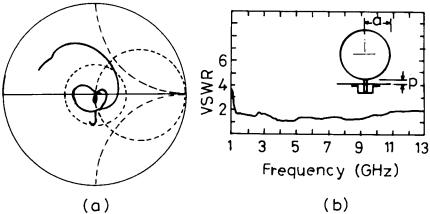
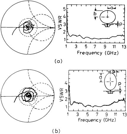
Figure 9.10 Measured (a) input impedance and (b) VSWR plots of CM antenna.
L = 2a |
(9.16) |
r = a /4 |
(9.17) |
For p = 0.1 cm, the measured input impedance and VSWR plots are shown in Figure 9.10. The BW for VSWR ≤ 2 is from 1.17 GHz to 12 GHz, which corresponds to a BW ratio of 1:10.2.
The BW of the CM is larger than all the monopole antennas described earlier. This could be interpreted in terms of various higher order modes of the circular patch. Unlike the various modes of rectangular resonator, modes of the circular resonator (characterized by the roots of the derivative of the Bessel function) are closely spaced as explained in Chapter 2. The BW associated with the various modes is very large because the disc is in the air; accordingly, the change in the input impedance from one mode to another mode is very small. This can also be noted from the impedance plot shown in Figure 9.10(a), which has multiple loops corresponding to the various modes. Since these loops are within the VSWR = 2 circle, a large BW is obtained.
9.5 Planar Elliptical Monopole Antennas
An elliptical monopole (EM) antenna is a generalized case of the circular monopole, wherein the major axis is not equal to the minor axis. The dimensions of EM (i.e., major axis length = 2a and minor axis length = 2b )
372 |
Broadband Microstrip Antennas |
are calculated, keeping its area equal to that of the CM. The ellipticity ratio is chosen as a /b . 1.1, which is named as EM1. The EM is fed either along the minor axis (EMA) or the major axis (EMB) as shown in the insets of Figure 9.11.
For calculating f L of the EM antenna, the L and r of the effective cylindrical monopole are determined by equating its area as:
2prL = p ab |
(9.18) |
For EMA, L = 2b and r = a /4, and for EMB, these parameters are L = 2a and r = b /4. The f L is calculated using (9.8).
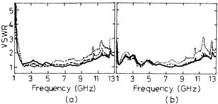
Figure 9.11 Measured input impedance and VSWR plots of (a) EM1A and (b) EM1B.
Broadband Planar Monopole Antennas |
373 |
The measured input impedance and VSWR plots for EM1A and EM1B are shown in Figures 9.11. The performances of these configurations are compared with those of the CM in Table 9.3. Improved VSWR BWs are obtained for EM1A and EM1B as compared to CM. Therefore, the effect of varying the ellipticity ratio on the BW of the EM antenna is described in Section 9.5.1.
9.5.1 Effect of Ellipticity Ratio
Three elliptical disc monopoles with different ellipticity ratios are considered by keeping the area same as before. For these three monopoles, the values of a /b are chosen as 1.2 (EM2), 1.3 (EM3), and 1.4 (EM4) [3].
The measured VSWR plots of EM2, EM3, and EM4 in configurations ‘‘A’’ and ‘‘B’’ are compared in Figure 9.12. The dimensions and measured VSWR BWs for all these cases are summarized in Table 9.3. The f L of EMBs is always smaller than that of the EMAs because of its larger height. As the ellipticity ratio a /b increases from 1.1 to 1.4, BW decreases. In comparison with the measured f L , the theoretical f L obtained using (9.18) and (9.8) is within ± 7.5% for most of the cases as shown in Table 9.3.
9.5.2 Radiation Pattern of Circular and Elliptical Monopole Antennas
Among all these broadband monopole configurations, the CM and EM1A antennas provide a maximum BW. The measured radiation patterns of these
Table 9.3
Comparison of VSWR BW of CM and Various EMs [3]
|
|
|
Measured |
|
|
|
|
a |
b |
Frequency |
Theoretical |
Percentage |
|
Configuration |
(cm) |
(cm) |
Range (GHz) |
f L (GHz) |
Error in f L |
|
CM |
2.5 |
2.5 |
1.17 |
to 12.0 |
1.258 |
+7.5 |
EM1A |
2.6 |
2.4 |
1.21 |
to 13* |
1.297 |
+7.2 |
EM1B |
2.6 |
2.4 |
1.20 |
to 12.50 |
1.220 |
+1.7 |
EM2A |
2.7 |
2.3 |
1.38 |
to 11.49 |
1.340 |
−2.9 |
EM2B |
2.7 |
2.3 |
1.13 |
to 12.00 |
1.185 |
+4.9 |
EM3A |
2.8 |
2.2 |
1.37 |
to 11.30 |
1.385 |
+1.1 |
EM3B |
2.8 |
2.2 |
1.08 |
to 11.43 |
1.152 |
+6.7 |
EM4A |
2.9 |
2.1 |
1.58 |
to 10.45 |
1.433 |
−9.3 |
EM4B |
2.9 |
2.1 |
1.09 |
to 10.45 |
1.121 |
+2.8 |
|
|
|
|
|
|
|
*Gives VSWR < 2 above 13 GHz also.
374 |
Broadband Microstrip Antennas |
Figure 9.12 Measured VSWR plots of (a) EMA and (b) EMB for different a /b ratios: ( —— ) 1.2, ( - - - ) 1.3, and ( ? ? ? ) 1.4.
two configurations at frequencies 2.5 GHz and 9 GHz are shown in Figure
9.13.The results are summarized as follows:
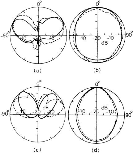
•At 2.5 GHz, the E-plane (elevation) pattern is conical, whereas the H-plane (azimuthal) pattern is nearly omni-directional with a maximum variation of 4 dB. The pattern is similar to that of a vertical 0.4l linear monopole antenna (which is approximately the equivalent height of the antenna at this frequency) on a finite ground plane.
•At 9 GHz, the effective height of the disc monopole is 3l/2, the E-plane pattern resembles to that of a 3l/2 vertical linear monopole antenna. The maximum variation of 7 dB is observed in the azimuthal pattern.
These patterns are similar to those of the thick monopole antennas on a finite ground plane, which round off the nulls of the pattern of the infinitesimal thin (very small radius) monopole on infinite ground plane and enhance the radiation at higher angles from the zenith [7, 8]. Slight distortions might be attributed to the shape of the planar monopole, reflections from metallic surfaces, and edge diffraction.
9.6 Design Examples of Monopole Antennas
Based upon the above discussions regarding the analysis of various monopole antennas, two design examples are presented.
Broadband Planar Monopole Antennas |
375 |
Figure 9.13 Radiation pattern of two monopole antennas at two frequencies: (a) E- and
(b) H-planes at 2.5 GHz and (c) E- and (d) H-planes at 9.0 GHz. [( —— ) CM and ( - - - ) EM1A.]
9.6.1 Monopole Antenna for 225–400 MHz
To cover the frequency range of 225–400 MHz for defense applications, an inverted disk cone monopole antenna is typically used; this is structurally not very convenient. Consequently, there is a need for a simple planar monopole antenna that can be easily fabricated and installed. This BW can be achieved with the planar RM antenna described in Section 9.2.