

256 Broadband Microstrip Antennas
7.2.1.3 Tunable RMSA with a Stub Along a Nonradiating Edge
In the above two cases, the stub(s) are placed along the radiating edge(s) of the RMSA, where the field remains constant. As a result, the position of the stub along the radiating edge does not have a significant effect on the tuning characteristics of the RMSA. When the stub is placed along one of the nonradiating edges of the RMSA, the position of the stub influences the input impedance and tunability characteristics of the antenna because of the sinusoidal field variation along the edge. A RMSA with a single stub placed along one of its nonradiating edges is shown in Figure 7.3. The position of the stub x s is varied from the center to the edge of the patch. For l = 1 cm, w = 0.4 cm, and x = 0.7 cm, the effect of x s on the performance of the antenna is summarized in Table 7.3. As x s increases from 0 to 1.3 cm, the resonance frequency decreases from 2.984 GHz to 2.793 GHz yielding a tuning range of 6.6%, while the input impedance Z in decreases from 71V to 36V, which decreases the BW from 66 to 25 MHz. However, when x s is moved from 0 to −1.3 cm, the resonance frequency variation is nearly same as before but the input impedance increases from 71V to 96V. Therefore, the input impedance of the antenna can be significantly controlled from 36V to 96V by moving the stub along the nonradiating edge from one extreme end to the other end.
7.2.1.4 Tunable CMSA with a Single Stub
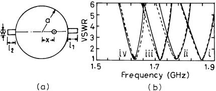
A coaxially fed CMSA with a single stub placed along the feed axis is shown in Figure 7.4(a). The improved transmission line model is used to analyze the antenna [6–8]. The radius of the CMSA is a = 3 cm, er = 2.33, h = 0.159 cm, and tan d = 0.001. For x = 0.95 cm, w = 0.4 cm, and different
Figure 7.3 RMSA with a stub along the nonradiating edge.

Tunable and Dual-Band MSAs |
257 |
Table 7.3
Effect of the Position x s of Stub Along the Nonradiating Edge of an RMSA
(L = 3 cm, W = 4 cm, l = 1 cm, w = 0.4 cm, x = 0.7 cm, er = 2.55, h = 0.159 cm, and tan d = 0.001)
xs |
f 0 |
Z in |
BW |
(cm) |
(GHz) |
(V) |
(MHz) |
|
|
|
|
0.0 |
2.984 |
71 |
66 |
0.5 |
2.940 |
53 |
58 |
1.0 |
2.853 |
37 |
39 |
1.3 |
2.793 |
36 |
25 |
−0.5 |
2.945 |
87 |
53 |
−1.0 |
2.858 |
95 |
34 |
−1.3 |
2.800 |
96 |
29 |
|
|
|
|
Figure 7.4 (a) CMSA with a single stub. (b) VSWR plots for various stub lengths l (i) 0, (ii) 1.2, (iii) 1.85, and (iv) 2.2 cm: ( - - - ) theoretical and ( —— ) measured.
stub lengths l (0 to 2.2 cm), the results are given in Table 7.4. The theoretical and measured VSWR curves for four different stub lengths are shown in Figure 7.4(b).
As l increases from 0.0 to 2.2 cm, the measured resonance frequency f 0 decreases from 1.868 GHz to 1.693 GHz, which yields a tuning range of nearly 9%. The increase in l increases the effective area of the CMSA, which decreases its resonance frequency. With an increase in the stub length, the effective center of the antenna shifts toward the feed point from the physical center. Therefore, the real part of the measured input impedance Z in decreases from 53.4V to 30.0V, and hence the BW decreases from 29 MHz to 9 MHz. The decrease in the BW is also due to the decrease of

258
|
|
|
|
Table 7.4 |
|
|
|
|
|
|
|
Theoretical and Experimental Results of a CMSA with a Single Stub for Various Values of Stub Length l |
|
||||||||
|
(a = 3 cm, w = 0.4 cm, x = 0.95 cm, er = 2.33, h = 0.159 cm, and tan d = 0.001) |
|
Broadband |
|||||||
l |
f 0 (GHz) |
|
|
Z in (V) |
|
|
BW (MHz) |
|||
(cm) |
Theoretical |
Experimental |
Theoretical |
Experimental |
Theoretical |
Experimental |
|
|||
|
|
|
|
|
|
|
|
|
Microstrip |
|
0.00 |
1.866 |
1.868 |
52.5 |
+ j 0.6 |
53.4 |
+ j 2.3 |
28 |
29 |
||
|
||||||||||
0.80 |
1.832 |
1.829 |
47.3 |
+ j 1.8 |
50.4 |
+ j 0.9 |
25 |
25 |
|
|
0.95 |
1.825 |
1.823 |
45.5 |
+ j 0.1 |
49.1 |
+ j 0.3 |
24 |
25 |
|
|
1.20 |
1.810 |
1.808 |
42.3 |
− j 1.9 |
45.5 |
− j 0.4 |
23 |
23 |
Antennas |
|
1.85 |
1.746 |
1.741 |
35.5 |
+ j 0.5 |
39.0 |
+ j 0.5 |
16 |
17 |
||
1.40 |
1.795 |
1.788 |
40.5 |
− j 0.1 |
44.0 |
− j 0.3 |
21 |
22 |
|
|
1.60 |
1.777 |
1.768 |
39.0 |
+ j 0.1 |
41.3 |
− j 0.2 |
18 |
19 |
|
|
2.00 |
1.733 |
1.723 |
30.7 |
− j 0.7 |
34.0 |
− j 0.8 |
13 |
15 |
|
|
2.10 |
1.717 |
1.711 |
28.9 |
+ j 0.1 |
30.5 |
+ j 0.6 |
10 |
11 |
|
|
2.20 |
1.695 |
1.693 |
28.0 |
+ j 0.1 |
30.0 |
+ j 1.0 |
8 |
9 |
|
|
|
|
|
|
|
|
|
|
|
|
|
Tunable and Dual-Band MSAs |
259 |
the resonance frequency, which effectively reduces h /l0. For a larger stub length, the feed point needs to be shifted away from the center for impedance matching, which will also improve the BW.
7.2.1.5 Tunable CMSA with Double Stubs
The CMSA with a single stub gives tunability, but the main disadvantage is that the same feed point does not give impedance matching for a larger stub length. The feed point needs to be moved away from the center to get a good match for longer stub. A CMSA with two stubs, shown in Figure 7.5(a) overcomes this problem [9]. When the two stubs are equal, then the configuration is symmetrical, and the effective center remains close to the physical center of the configuration. So, even for longer stub lengths, the feed point remains unchanged for a 50-V match. The theoretical and experimental resonance frequencies, input impedance and BW for VSWR ≤ 2 for different stub lengths l1 and l2 are given in Table 7.5. The theoretical and experimental VSWR plots for four different combinations of stub lengths are given in Figure 7.5(b). As the stub lengths (l1 and l2) increase from (0, 0) to (1.45, 1.70) cm, the measured resonance frequency decreases from 1.868 GHz to 1.696 GHz, leading to a tuning range of about 9%, whereas the real part of the input impedance decreases slightly from 53.4V to 50.0V. Also, the BW decreases from 29 MHz to 19 MHz, because the resonance frequency decreases, which decreases h /l0. When the difference between the two stub lengths increases, the change in the impedance is more.
Figure 7.5 (a) Double stub-loaded CMSA and (b) VSWR plots for various stub lengths (l1, l2) in centimeters [(i) (0, 0), (ii) (0.45, 0.95), (iii) (1.25, 0.95), and (iv) (1.45, 1.7)]: ( - - - ) theoretical and ( —— ) measured.

Table 7.5
Theoretical and Experimental Results of the Double Stub-Loaded CMSA for Different Stub Lengths l1 and l2 (a = 3 cm, x = 0.95 cm, er = 2.33, h = 0.159 cm, and tan d = 0.001)
Stub Lengths |
|
|
|
|
|
|
|
|
|
|
(cm) |
|
f 0 (GHz) |
|
Z in (V) |
|
|
|
BW (MHz) |
l1 |
l2 |
Theoretical |
Experimental |
Theoretical |
Experimental |
Theoretical |
Experimental |
||
0.00 |
0.00 |
1.866 |
1.868 |
52.5 |
+ j 0.6 |
53.4 |
+ j 0.3 |
28 |
29 |
0.45 |
0.40 |
1.826 |
1.832 |
53.0 |
+ j 1.8 |
53.6 |
− j 0.3 |
27 |
27 |
0.45 |
0.95 |
1.800 |
1.804 |
58.2 |
+ j 0.8 |
55.1 |
− j 0.1 |
26 |
24 |
1.25 |
0.95 |
1.760 |
1.763 |
50.7 |
+ j 0.9 |
48.1 |
+ j 0.9 |
22 |
21 |
1.25 |
1.45 |
1.725 |
1.732 |
57.6 |
+ j 0.3 |
53.0 |
+ j 0.4 |
21 |
19 |
1.45 |
1.45 |
1.710 |
1.721 |
54.7 |
+ j 1.5 |
50.0 |
+ j 0.4 |
20 |
20 |
1.45 |
1.70 |
1.699 |
1.696 |
51.5 |
− j 0.7 |
50.0 |
− j 0.5 |
19 |
19 |
|
|
|
|
|
|
|
|
|
|
260
Antennas Microstrip Broadband

Tunable and Dual-Band MSAs |
261 |
7.2.2 Tunable MSAs Using Shorting Posts
When a shorting post is placed between the patch and the ground plane, it changes the field distribution and provides inductive loading to the patch and hence changes its resonance frequency. The resonance frequency can be tuned by changing the position and the number of shorting posts in the patch. As discussed in Chapter 6, the conventional MSAs, such as the RMSA, CMSA, and ETMSA, are made compact by shorting the zero potential field lines and using part of the configuration. It is also described that by reducing the shorting width or number of shorting posts, the resonance frequency decreases, thereby achieving tuning.
An RMSA of length L = 1.2 cm and W = 1.2 cm with shorting posts placed along one of its radiating edges is shown in Figure 7.6(a) [10]. The feed point is at x = 0.155 cm, and the substrate parameters are er = 2.55 and h = 0.12 cm. The variation of normalized frequency f /f 0 with respect to the shorting ratio ws /W (ratio of width of the shorted portion to the width of the patch) is shown in Figure 7.6(b). As the shorting ratio decreases from 1.0 to 0.1, the normalized resonance frequency decreases from 1.0 to 0.65, which is similar to that described in Section 6.2.
Another configuration for tuning the resonance frequency of the RMSA by using two shorting posts inside the patch is shown in Figure 7.7(a) [10, 11]. The dimensions of the RMSA are L = 6.2 cm and W = 9.0 cm, and the substrate parameters are er = 2.55 and h = 0.16 cm. For the feed at x = 1.6 cm along the nonradiating edge, the variation of the frequency with s ′/L
Figure 7.6 (a) RMSA with shorting posts placed along one of its radiating edges and (b) its normalized frequency f /f 0 variation with the shorting width ratio w s /W : ( - - - ) theoretical and ( —— ) measured.

262 |
Broadband Microstrip Antennas |
Figure 7.7 (a) RMSA with two shorting posts and (b) its frequency variation with s ′/L : ( - - - ) theoretical and ( —— ) measured.
ratio (separation of the two shorting posts to the length of the patch) is shown in Figure 7.7(b). As s ′/L increases (i.e., the two shorting posts are shifted away from the center to the edge of the patch), the measured resonance frequency increases and then decreases slightly, and a tuning range of approximately 18% is obtained. The radiation pattern remains in the broadside direction.
7.2.3 Tunable MSAs Using Varactor Diodes
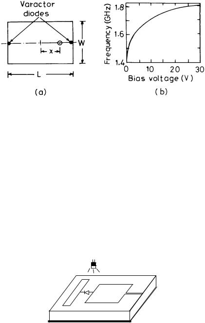
Instead of using two shorting posts, which provide inductive loading to the patch for tuning its resonance frequency, two varactor diodes are connected at the two radiating edges of the patch to the ground plane, as shown in Figure 7.8(a). The dimensions of the patch are L = 4.65 cm and W = 3.0 cm and the feed point is located at x = 1.7 cm. Frequency tuning is achieved by varying the reverse-bias voltage applied to the varactor diodes. The plot of measured resonance frequency versus reverse-bias voltage (V) is shown in Figure 7.8(b). With an increase in the reverse-bias voltage, the diode capacitance decreases, which decreases the overall capacitance of the patch; hence the resonance frequency of the antenna increases. Due to the nonlinear behavior of the varactor capacitance with bias voltage, frequency variation is not linear with bias voltage. As the bias voltage is increased from 0 to 30V, the frequency increases from 1.40 GHz to 1.81 GHz, giving a tuning range of about 30% [12].
Tunable and Dual-Band MSAs |
263 |
Figure 7.8 (a) RMSA with two varactor diodes and (b) plot of measured resonance frequency versus reverse-bias voltage.
7.2.4 Optically Tuned MSA
Another configuration for tuning the resonance frequency of the MSA uses an optically controlled PIN diode as depicted in Figure 7.9. A stub is connected or disconnected to the patch by means of an optically controlled PIN diode depending upon whether the diode is forward-biased or reversebiased, respectively. When the diode is reverse-biased, its impedance is high; it acts as an open circuit; and the resonance frequency of the antenna corresponds to the patch frequency. When the diode is forward-biased, its impedance is low, and the resonance frequency corresponds to the combination of the patch and the stub [13].
7.2.5 Tunable MSAs Using an Air Gap
The above planar methods provide a frequency tuning range of 5–30%, but one has to add external components, such as stubs, shorting posts, varactor
Figure 7.9 RMSA with an optically controlled PIN diode.

264 |
Broadband Microstrip Antennas |
diodes, an optically controlled PIN diode, and their associated biasing circuits [1]. Another method for tuning the resonance frequency of the MSA, which avoids the placement of the external components, is to change the effective dielectric constant ee of the antenna by introducing an adjustable air gap between the substrate and the ground plane as shown in Figure 7.10. By varying the air gap D, the resonance frequency of the MSA is tuned. A similar configuration is discussed in Chapter 2 for a broad BW for fixed air gap. As D increases, eeq decreases as given by (2.25), which increases the resonance frequency. Also, the BW of the antenna increases due to an increase in the total height H = h + D and a decrease in eeq .
A circular patch of radius a = 5 cm is fabricated on a substrate with er = 2.32 and h = 0.159 cm. Spacers are used between the substrate and the ground plane to maintain an air gap as shown in Figure 7.10. The patch is fed at x = 4.75 cm. For D = 0, 0.05 and 0.1 cm, the measured resonance frequencies for the fundamental mode are 1.128, 1.286, and 1.350 GHz, respectively. This gives a frequency tuning range of about 20%. The BW of the antenna increases from 0.89% to 2.07% due to an increase in the total height of the antenna and a decrease in ee . There is no significant effect of the air gap on the radiation pattern of the antenna. Similar results are also observed for higher order modes of the CMSA [14, 15].
Instead of a CMSA, when an ARMSA with an outer radius of 7.0 cm and an inner radius of 3.5 cm is used, its resonance frequency for the fundamental TM11 mode is 626, 720, and 778 MHz for D = 0.0, 0.05, and 0.1 cm, respectively [16]. BWs at these frequencies are 0.6%, 0.7%, and 0.8%, respectively. For the TM12 mode, the corresponding resonance frequencies are 2.757, 3.040, and 3.240 GHz, with respective BWs of 4.0%, 8.0%, and 8.6%.
A simple formula for calculating the resonance frequency f gap of a patch with small air gap spacing D is as follows:
|
|
f gap = |
f 0 |
√ |
er |
|
(7.4) |
|||||||
|
|
|
|
|
||||||||||
|
|
|
|
|
||||||||||
|
|
|
√eeq |
|||||||||||
|
|
|
|
|
|
|
|
|
|
|
|
|
|
|
|
|
|
|
|
|
|
|
|
|
|
|
|
|
|
|
|
|
|
|
|
|
|
|
|
|
|
|
|
|
|
|
|
|
|
|
|
|
|
|
|
|
|
|
|
|
|
|
|
|
|
|
|
|
|
|
|
|
|
|
|
|
|
|
|
|
|
|
|
|
|
|
|
|
|
|
|
|
|
|
|
|
|
|
|
|
|
|
|
|
Figure 7.10 Tunable MSA with an air gap between the substrate and the ground plane.
Tunable and Dual-Band MSAs |
265 |
where f 0 is the resonance frequency of the patch without any air gap and eeq is the effective dielectric constant of the two layers given by (2.25). The above equation is valid for small values of D and any patch shape.
7.2.6 Tunable MSAs Using a Ferrite Substrate
A ferrite substrate has a large permeability mr and high dielectric constant er . When an RMSA is fabricated on a ferrite substrate, its resonance frequency is given by
|
c |
||
f 0 = |
|
|
(7.5) |
|
|
||
|
|
||
|
2L e √me ee |
||
where me is the effective permeability.
Because of its large value in the lower UHF band, the size of the patch on a ferrite substrate reduces drastically for a given frequency. A fully shorted quarter-wave RMSA with L = 4 cm, W = 1.12 cm, and a feed point at x = 1.12 cm from the open end is fabricated on a ferrite substrate, whose parameters are h = 0.2 cm, mr = 14.74, er = 15, dielectric loss tangent factor = 0.0476, and magnetic loss tangent factor = 0.0476. The measured BW of the antenna is 7 MHz (3.2%) at 219 MHz for VSWR ≤ 1.5 [17]. When a CMSA of radius a = 1 cm and x = 0.5 cm is fabricated on the above ferrite substrate, it has a resonance frequency of 661 MHz. The antenna yielded wider BW of 12.4% for VSWR ≤ 1.5 because of increase in h /l0 [18].
When a ferrite substrate experiences a varying magnetic field, its permeability changes, which yields frequency tuning. An RMSA of L = 1.4 cm and W = 1.8 cm is fabricated on a ferrite substrate with h = 0.127 cm, er = 15 and 4p Ms = 1,720 Gauss [19]. The RMSA is fed at the middle of one of the radiating edges for the TM10 mode. The tuning of the resonance frequency is achieved by varying the dc magnetic bias field, which is realized by placing a permanent magnet behind the ground plane of the MSA. The strength of the magnetic field is changed by adjustable spacers. The tuning range of 40% is achieved at 4.6 GHz for VSWR ≤ 2. The radiation pattern remains in the broadside direction with cross-polar level less than −10 dB in the complete tuning range.
The continuous tuning of the resonance frequency of the MSA over the large frequency range is also possible by changing the biasing current of the electromagnet placed below its ground plane as shown in Figure 7.11 [20]. The electromagnet is biased by setting the current through the fixed