Results of calculation

Graphical dependences of calculated currents through the branches of the given circuit (fig. 8.1.) accord to the every iteration step is represented in the figure 8.4.

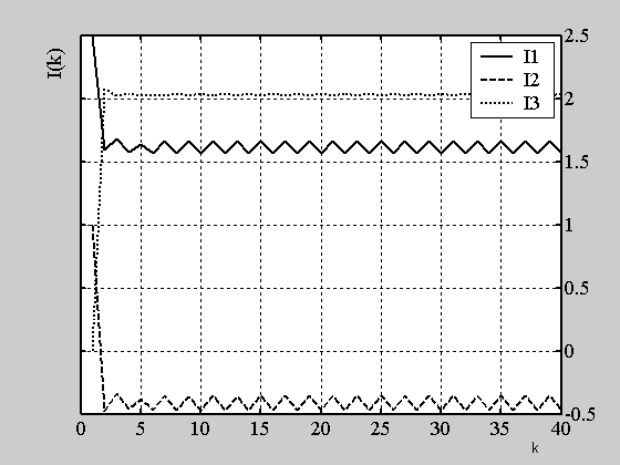
Figure 8.4 – Calculated of the currents through the branches

The iteration series of the approached solutions make cyclical oscillations around of a required solution and it is mapped by the above-represented graphical dependences. It is obvious, that this process is divergent.

Improvement of convergence of the Newton method

To improve convergence the weight coefficient for calculated values of the currents through the branches is applied. We shall make the following modifications to the main program:

% branch currents

I (3, k) = (J0-phi (1) *G0+I (3, k-1)) *0.5;

I (1, k) = (J1k+phi (1) *G1k+I (1, k-1)) *0.5;

I (2, k) = (J2k + (phi (2)-phi (1)) *G2k+I (2, k-1)) *0.5;

Arrive as result calculated graphical dependences of currents through the branches. If convergence is unsatisfactory, reduce a weight value of a new approximation as follows:

% branch currents

I (3, k) = (J0-phi (1) *G0+3*I (3, k-1)) *0.25;

I (1, k) = (J1k+phi (1) *G1k+3*I (1, k-1)) *0.25;

I (2, k) = (J2k + (phi (2)-phi (1)) *G2k+3*I (2, k-1)) *0.25;

Arrive as result calculated graphical dependences of currents through the branches for every iteration step as function of iteration number. Be convinced, that process is convergent.

The task for fulfillment

 Study item 8.1.

 Repeat the program considered in item. 8.2 and arrive as result calculated graphical dependences of currents through the branches for every iteration step as function of iteration number. (Fig 8.4);

 According to item. 8.3 achieve convergence of process of evaluations. Arrive as result calculated graphical dependences of convergence of process of evaluations of currents through the branches.

 Laboratory work results (the program, listing of calculation, graphics) are saved in a personal file.

 Draw up the report on laboratory work. The report would contain the mathematical model of the studied circuit, texts of programs, results of calculation, conclusions.

9 LAboratory work # 9

TOPIC : Modeling of electromagnetic processes in magnetic circuits of a direct magnetic flux in MATLAB environment. Part 1.

PURPOSE OF THE WORK: Problem statement, development of the program of calculation of a nonlinear magnetic circuit by the Newton method using discrete models of nonlinear resistance and their spline-interpolation.

Mathematical model

Let's make mathematical model of the magnetic circuit (Fig. 9.1) in MATLAB environment if all nonlinear components are given by discrete models, and their curves of magnetization as reference points.

Figure 9.1 - Modeled magnetic circuit

Let parameters of a circuit are given:

Length of average magnetic lines according to fig. 9.1:

l1=0.3 m; l2=0.3 m; l3=0.1 m;

Breadth of magnetic limbs:

D1=0.1 m; D2=0.1 m; D3=0.1 m;

Thickness of the core:

dlt=0.1 m;

Magnitude of the air-gap:

Luft=0.00002 m;

Current and loops of windings:

I=1 A; N=20.

Curve of magnetization of core B (H) is shown in figure 9.2.

а).

b).

а) – general view;

b) – an initial section of the magnetization curve.

Figure 9.2 – Magnetization curve B(H) of the core steel

An equivalent circuit of the given magnetic circuit is represented in fig. 9.3.

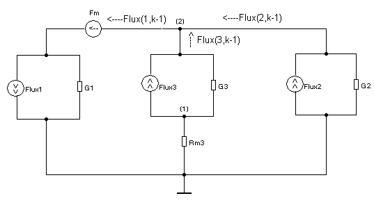
Figure 9.3 – The equivalent circuit

According to the second Kirchhoff law it is possible to transfer MMF source Fm into a branch containing conductance G1 and then to transform it to a source of magnetic flux FmG1. The equivalent circuit according to these transformations is offered in fig. 9.4.

Figure 9.4 – The equivalent transformed circuit with magnetic flux source FmG1