

prt%3A978-0-387-35973-1%2F16
.pdfMobile Usage and Adaptive Visualization |
681 |
trol the adaptation method. The output of the adaptation method is a set of adapted objects. For the adaptation of the visualization of geographic information to the mobile usage context, the following adaptation methods are applicable:
¥Selection method: this method selects map features depending on the usage context in order to reduce the map content and the information density. This method operates as a kind of Þlter. The Þlter criterion can be a spatial relation as in the case of LBS, or it could be a user preference stored in a user proÞle.
¥Prioritization method: this method classiÞes the priority of selected information items with regard to the current usage context. The priority classes are based on the relevance of the information for different context factors, e. g., relevance for the current location or relevance for the current activity.
¥Substitution method: this method substitutes one visualization form with an equivalent presentation form. A map could, for instance, be substituted by an image or abstract symbols might be replaced by pictorial symbols.
¥Symbolization method: this method changes the symbolization of the visual elements by applying a different symbol style or by switching to a predeÞned design alternative.
¥ConÞguration method: this method conÞgures or reconÞgures visual components in order to adjust the visualization to the usage context. For instance a different base map or a different scale might be selected depending on mobility-related factors such as means of transport or movement speed. The conÞguration method could also conÞgure the user interface through hiding or aggregating functions or changing interaction modes.
¥Encoding method: this method changes the encoding of the information (e. g., vector to raster) to be transmitted to a mobile device in dependence on technological factors such as the bandwidth available or the capabilities of the device.
In the simplest case, a Þxed rule base exists that triggers the adaptation methods and states what changes will be applied if speciÞc context conditions are given. More advanced adaptive systems incorporate a learning component that dynamically changes the knowledge base in dependence on the system usage and performed user interactions.
Key Applications
Adaptive visualization, so far, is used mainly in the domain of mobile systems and services. The domains discussed here are mobile guide systems, LBS, and mobile geospatial web services.
Mobile Guide Systems |
|
|
The adaptivity principle has been applied in many mobile |
|
|
guide systems [8,9]. The visualization in such guide sys- |
|
|
tems is either adapted to the user characteristics or prefer- |
|
|
ences (personalization) or to the usage context factors in |
|
|
general. |
|
|
Location-Based Services |
|
|
LBS are inherently adaptive by spatially Þltering informa- |
|
|
tion for a speciÞed location [10]. Different ways of adapt- |
|
|
ing LBS are described in [11]. |
|
|
Mobile Geospatial Web Services |
|
|
Most mobile geospatial web services include maps or other |
|
|
forms of visualization of geographic information to assist |
|
|
the user in way-Þnding, orientation or similar spatial tasks. |
|
|
Adaptive visualizations are employed in such services to |
|
|
improve their usability [7]. |
|
|
Future Directions |
|
|
In principle, any visualization of geographic information |
|
|
M |
||
can be adapted to the context of use. With the growing |
||
amount of geospatial data available the demand for the |
|
|
adaptation to speciÞc needs and contexts will probably get |
|
|
stronger in the near future. |
|
|
The adaptivity principle is especially important for the |
|
|
evolving mobile geospatial web services and their inter- |
|
|
faces where usability is a crucial issue. A thoughtful imple- |
|
|
mentation of adaptive behavior helps to reduce complexi- |
|
|
ty and take some of the cognitive load inherent in mobile |
|
|
usage contexts. Adaptive visualization will play an impor- |
|
|
tant role in personalized geospatial web services and ego- |
|
|
centric maps [12]. |
|
Cross References
Visualizing Constraint Data
Web Services, Geospatial
Recommended Reading
1.Reichenbacher, T.:, Mobile Cartography Adaptive Visualisation of Geographic Information on Mobile Devices. Verlag Dr. Hut, Munich (2004)
2.Browne, D., Totterdell, P., Norman, M. (eds.): Adaptive user interfaces. Academic Press, London (1990)
3.Oppermann, R. (ed.): Adaptive user support: ergonomic design of manually and automatically adaptable software. Lawrence Erlbaum, Hillsdale, NJ (1994)
4.Schneider-Hufschmidt, M., KŸhme, T., Malinowski, U.(eds.): Adaptive user interfaces: principles and practice. North-Holland, Amsterdam (1993)

682 MOBR
5.Brusilovsky, P.: Adaptive hypermedia. User Model. User-Adapt. Interact. 11, 87Ð110 (2001)
6.Dey, A.K.: Understanding and using context. Personal Ubiquitous Comput. J. 5, 4Ð7 (2001)
7.Sarjakoski, T., Nivala A.-M.: Adaptation to context Ñ a way to improve the usability of mobile maps. In: Meng, L., Zipf, A., Reichenbacher, T. (eds.) Map-Based Mobile Services. Theories, Methods and Implementations, pp. 7Ð123. Springer, Heidelberg (2005)
8.Oppermann, R., Specht, M.: Adaptive mobile museum guide for information and learning on demand, in human-computer interaction. In: Bullinger, H.J., Ziegler, J. (eds.). Proceedings of HCI International Õ99, vol. 2: Communication, Cooperation, And Application Design, pp. 642Ð646. Erlbaum, Mahwah (1999)
9.Patalaviciute, V., et al.: Using SVG-based Maps for Mobile Guide SystemsÑA Case Study for the Design, Adaptation, and Usage of SVG-based Maps for Mobile Nature Guide Applications. (2005) Available via http://www.svgopen.org/2005/papers/ MapsForMobileNatureGuideApplications/index.html
10.Krug, K., Mountain, D., Phan, D.: Location-based services for mobile users in protected areas. Geoinformatics, 6(2), 26Ð29 (2003)
11.Steiniger, S., Neun, M., Edwardes, A.: Foundations of Location Based Services (2006). Available via http://www.geo.unizh.ch/ publications/cartouche/lbs_lecturenotes_steinigeretal2006.pdf
12.Reichenbacher, T.: Adaptive egocentric maps for mobile users. In: Meng, L., Zipf, A., Reichenbacher, T. (eds.) Map-Based Mobile Services. Theories, Methods and Implementations, pp. 141Ð158. Springer, Heidelberg (2005)
MOBR
Minimum Bounding Rectangle
Model Driven Architecture
Modeling with Enriched Model Driven Architecture
Model Driven Development
Modeling with Enriched Model Driven Architecture
Model Driven Engineering
Modeling with Enriched Model Driven Architecture
Model Generalization
Abstraction of GeoDatabases
Modeling and Multiple Perceptions
CHRISTINE PARENT1, STEFANO SPACCAPIETRA2,
ESTEBAN ZIMçNYI3
1University of Lausanne, Lausanne, Switzerland
2Swiss Federal Institute of Technology, Lausanne, Switzerland
3Free University of Brussels, Brussels, Belgium
Synonyms
Data modeling; Multiscale databases; Multirepresentation
Definition
Multirepresentation generalizes known concepts such as database views and geographic multiscale databases. This chapter describes the handling of multi-representation in the MADS (Modeling Application Data with Spatio-tem- poral features) data modeling approach. MADS builds on the concept of orthogonality to support multiple modeling dimensions. The structural basis of the MADS model is based on extended entity-relationship (ER) constructs. This is complemented with three other modeling dimensions: space, time, and representation. The latter allows the speciÞcation of multiple perceptions of the real world and modeling of the multiple representations of real-world elements that are needed to materialize these perceptions.
Historical Background
Traditional database design organizes the data of interest into a database schema, which describes objects and their relationships, as well as their attributes. At the conceptual level, the design task relies on well-known modeling approaches such as the ER model [1] and UniÞed Modeling Language (UML) [2]. These approaches only deal with classical alphanumeric data. The idea of using conceptual spatial and spatiotemporal data models emerged in the 1990s. Most proposals were extensions of either the ER (e. g., [3,4,5]), UML (e. g., [6,7]), or object-oriented data models (e. g., [8]). Spatiotemporal data models are the current focus of research and development, both in academia and in industry: They allow the representation of the past and future evolution of geographic objects as well as moving and deforming objects. Both features are essential for complex development issues such as environmental management and city planning.
Most geographic applications confronted with a variety of user categories showing different requirements of the same data (e. g., different administrations involved in city management) also need another modeling dimension: multiple
Modeling and Multiple Perceptions |
683 |
representations. Multiple representations allow, for example, the spatial feature of a city being described as a point and as an area, the former for use in statewide maps, the latter in local maps. Interest in supporting this functionality has emerged recently [5,9] and the concept of multirepresentation is now popular in the research community and with user groups. The MADS proposal is playing an important role in establishing and advancing this trend.
Scientific Fundamentals
Definition 1: conceptual data model. A data model is conceptual if it enables a direct mapping between the perceived real world and its representation with the concepts of the model. In particular, a conceptual model does not have implementation-related concerns.
Definition 2: data modeling dimension. A data modeling dimension is a domain of representation of the real world that focuses on a speciÞc class of phenomena. Examples of modeling dimensions include: data structure, space, time, and multirepresentation.
Definition 3: orthogonality. Modeling dimensions are said to be orthogonal if, when designing a database schema, choices in a given dimension do not depend on the choices in other dimensions. For example, it should be possible to record the location of a reservoir on a river (a spatial feature in the space dimension) irrespective of whether the reservoir, in the data structure dimension, has been modeled as an independent object or as an attribute of the river object. Orthogonality greatly simpliÞes the data model and its use, while enhancing its expressive power, i. e., its ability to represent all phenomena of interest. The orthogonality of multiple modeling dimensions is an essential characteristic of MADS. A detailed presentation of the model can be found in [5,10].
Modeling and Multiple Perceptions, Figure 1 A diagram of an object type with its attributes
Thematic Data Structure Modeling |
|
||
Definitions 4, 5, and 6: Object Types, Attributes, and |
|
||
Methods Database objects represent real-world entities |
|
||
of interest to applications. An object type deÞnes the prop- |
|
||
erties of interest for a set of objects that, from the appli- |
|
||
cation viewpoint, are considered as similar. Properties are |
|
||
either attributes or methods. An attribute is a property |
|
||
that is represented by a value in each object of the type. |
|
||
A method is a behavioral property common to all objects |
|
||
of the type. |
|
|
|
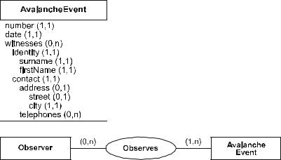
Figure 1 illustrates an object type AvalancheEvent and |
|
||
its attributes. These may |
be simple, e. g., number for |
|
|
AvalancheEvent, or complex (i. e., composed of other |
|
||
attributes), e. g., witnesses. |
|
||
Definition 7: Cardinality |
Attribute cardinality, deÞned |
|
|
by two numbers (min, max), denotes the minimum and |
|
||
maximum number of values that an attribute may hold |
|
||
within an object. The maximum cardinality determines |
|
||
whether an attribute is monovalued or multivalued, i. e., |
|
||
whether it holds at most one or several values. The mini- |
|
||
mum cardinality determines whether an attribute is option- |
|
||
al (min = 0) or mandatory (min > 0), i. e., whether an |
|
||
M |
|||
object may hold no value or must hold at least one value. |
|||
|
|
|
|
Definitions 8 and 9: Relationship Types and Roles
Relationships represent real-world links between objects that are of interest to the application. Relationships that, from the application perspective, have the same characteristics are grouped in relationship types. Roles represent the involvement of an object type into a relationship type. A relationship type deÞnes two or more roles: They are n- ary, n being the number of roles. Figure 2 shows an example of a binary relationship of the type Observes.
Cardinality constraints deÞne the minimum and maximum number of relationships that may link an object in a role. For example, in Fig. 2 the (0,n) cardinalities on the role associated to the Observer object type express that an observer may have never observed an avalanche, and that an observer may have observed any number of avalanches. As object types, relationship types may be described by properties (attributes and methods). The generic term instance denotes either an object or a relationship: an object (relationship) is an instance of the object (relationship) type it belongs to. MADS identiÞes two basic kinds of relationship types, association and multiassociation, described next.
Modeling and Multiple Perceptions, Figure 2 A diagram showing a relationship type linking two object types
684 Modeling and Multiple Perceptions
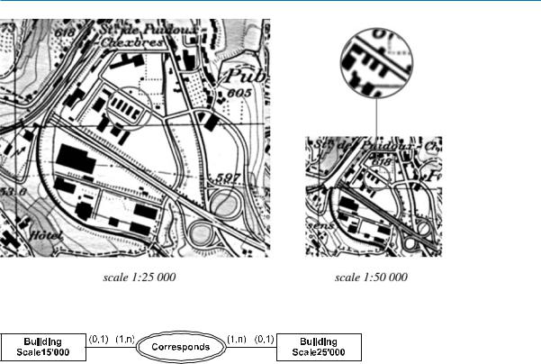
Modeling and Multiple Perceptions, Figure 3 An example situation calling for a multiassociation relationship
Modeling and Multiple Perceptions, Figure 4 An example of a multiassociation type
Definition 10: Association Types An association type is a relationship type such that each role links exactly one instance of the linked object type.
Associations are the usual kind of relationships. However, in some situations the association relationship does not allow accurate representation of real-world links existing between objects. Figure 3 shows two maps of the same area at different scales. Focusing on the area within the superimposed circles, the left-hand, more detailed, map shows Þve aligned buildings whereas at the same location the right-hand map shows only three. Suppose that the application stores the Þve buildings in the left-hand map as instances of the BuildingScale15’000 object type, and the three buildings in the right-hand map as instances of the BuildingScale25’000 object type. If the application requires the correlation of cartographic representations, at different scales, of the same real-world entities, some link must relate the Þve instances of BuildingScale15’000 to the three instances of BuildingScale25’000. The multiassociation construct allows directly representation of such a link.
Definition 11: Multiassociation Types A multiassociation type is a relationship type such that each role links a nonempty collection of instances of the linked object type.
Consequently, each role in a multiassociation type bears two pairs of (min, max) cardinalities. A Þrst pair is the conventional one, deÞning for each object instance how many relationship instances it can be linked to via the role. The second pair deÞnes for each relationship instance how many object instances it can link with this role. Its value for minimum is at least 1. Using a multiassociation type, the above correspondence between cartographic buildings can be modeled as shown in Fig. 4.
Apart from the additional cardinality constraints, multiassociation types share the same features as association types.
Definition 12: is-a Links The is-a (or generalization/specialization) link relates two object or two relationship types, a generic one (the supertype) and a speciÞc one (the subtype). It states that the subtype describes a subset of the real-world instances described by the supertype, and this description is a more precise one.
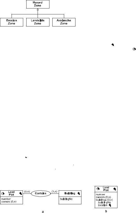
Figure 5 shows a generalization hierarchy of object types with three is-a links. The generic object type representing hazard zones is specialized in subtypes representing landslide, erosion, and avalanche zones.
A well-known characteristic of is-a links is property inheritance: All properties and links deÞned for the supertype also hold for the subtype. An immediate beneÞt of inher-
Modeling and Multiple Perceptions |
685 |
Modeling and Multiple Perceptions, Figure 5 Object types connected by is-a links
itance is type substitutability, i. e., enforcing the fact that wherever an instance of a type can be used in some data manipulation, an instance of any of its subtypes can be used instead.
Describing Space and Time Using the Discrete View
In MADS, space and time description is orthogonal to data structure description, which means that the description of a phenomenon may be enhanced by spatial and temporal features whatever data structure (i. e., object, relationship, attribute) has been chosen to represent it.
Definition 13: Discrete View The discrete (or object) view of space and time deÞnes the spatial and temporal extents of the phenomena of interest. The spatial extent is the set of points that the phenomenon occupies in space, while the temporal extent is the set of instants that it occupies in time.
SpeciÞc data types support the manipulation of spatial and temporal values, like a point, a surface, or a time instant. MADS supports a hierarchy of spatial data types and another hierarchy of temporal data types. Generic data types allow the description of object types whose instances may have different types of spatial or temporal extents. For example, a River object type may contain large rivers with an extent of type Surface and small rivers with an extent of type Line. Examples of spatial data types are: Geo ( ), the most generic spatial data type, Surface (
 ), and SurfaceBag (
 ). The latter is useful for describing objects with a nonconnected surface, like an archipelago. Examples of temporal data types are: Instant (
 ),
),
TimeInterval ( ), and IntervalBag (
 ). The latter is useful for describing the periods of activity of noncontinuous phenomena.
In MADS, temporality associated to object/relationship types or to attributes corresponds to valid time, which conveys information on when a given fact of the database is considered valid from the application viewpoint.
Definition 14: Spatial, Temporal, Spatiotemporal |
|
|
Objects and Relationships A spatial (and/or temporal) |
|
|
object type is an object type that holds spatial (and/or tem- |
|
|
poral) information pertaining to the object as a whole. |
|
|
For example, in Fig. 6a both object types are spatial as |
|
|
shown by the Surface ( ) icon, while only LandPlot is |
|
|
temporal as shown by the TimeInterval ( ) icon. Follow- |
|
|
ing common practice, an object type is called spatiotempo- |
|
|
ral if either it has both a spatial and a temporal extent, sep- |
|
|
arately, or has a time-varying spatial extent (i. e., its spatial |
|
|
extent changes over time and the history of extent values |
|
|
is recorded). |
|
|
Similarly, spatial, temporal, and spatiotemporal relation- |
|
|
ship types hold spatial and/or temporal information per- |
|
|
taining to the relationship as a whole, as for an object type. |
|
|
For example, in Fig. 2, the Observes relationship type |
|
|
can be deÞned as temporal, of the type Instant, to record |
|
|
when observations are made. |
|
|
M |
||
Spatial and temporal information at the objector rela- |
||
tionship-type level is kept in dedicated system-deÞned |
|
|
attributes: geometry for space and lifecycle for time. |
|
|
Geometry is a spatial attribute (see below) with any spatial |
|
|
data type as domain. When representing a moving object, |
|
|
geometry is a time-varying spatial attribute. On the other |
|
|
hand, the lifecycle allows users to record when an object |
|
|
(or link) was (or is planned to be) created and deleted. It |
|
|
may also support recording that an object is temporarily |
|
|
suspended, like an employee who is on temporary leave. |
|
|
Therefore the lifecycle of an instance says for each instant |
|
|
what is the status of the corresponding real-world object |
|
|
(or link) at this instant: scheduled (its creation is planned |
|
|
later), active, suspended (it is temporarily inactive), dis- |
|
|
abled (deÞnitively inactive). |
|
|
Definition 15: Spatial, Temporal, Spatiotemporal Attri- |
|
|
butes A spatial (temporal) attribute is a simple attribute |
|
|
whose domain of values is one of the spatial (tempo- |
|
|
ral) data types. A spatiotemporal attribute is a time- |
|
Modeling and Multiple Perceptions, Figure 6 a, b Alternative schemas for land plots and buildings
686 Modeling and Multiple Perceptions
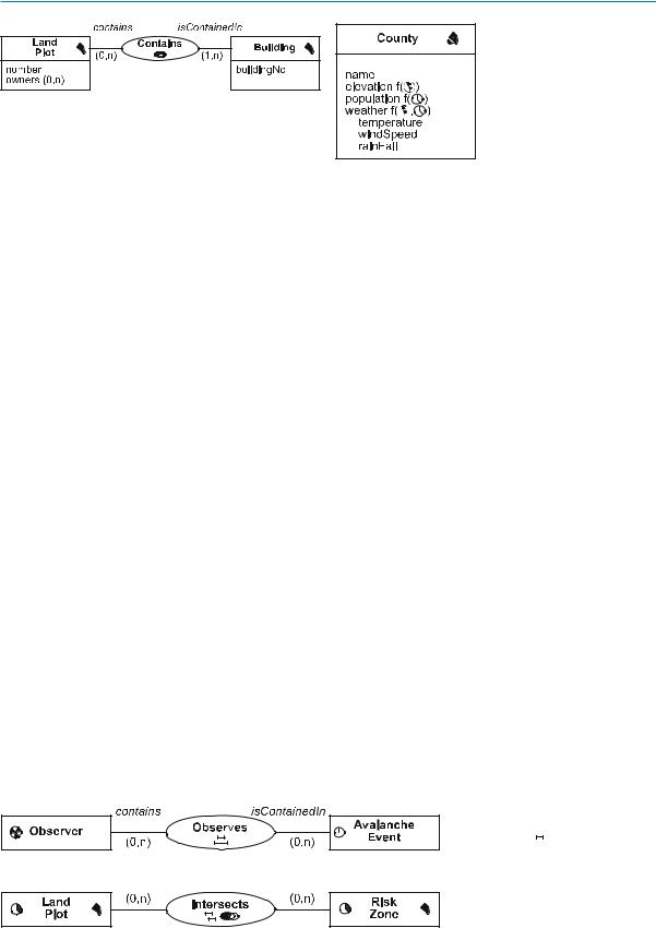
Modeling and Multiple Perceptions, Figure 7 A topological relationship of the type Inclusion ( )
)
varying spatial attribute, i. e., a spatial attribute whose value changes over time and the history of its values is recorded (see DeÞnition 17).
Each object and relationship type, whether spatiotemporal or not, may have spatial, temporal, and spatiotemporal attributes. For example, in Fig. 6b the LandPlot object type includes, in addition to its spatial extent, a complex and multivalued attribute buildings whose second component attribute, location, is a spatial attribute describing, for each building, its spatial extent.
Constraining Relationships with Space and Time Predicates
The links among spatial (temporal) object types often describe a spatial (temporal) constraint on the spatial (temporal) extents of the linked objects. For example, designers may want to enforce each Contains relationship of Fig. 6a to link a pair of objects provided that the spatial extent of the land plot contains the spatial extent of the building. In MADS, this can be done by deÞning Contains as a constraining relationship of the type topological inclusion, as shown in Fig. 7 by the  icon.
icon.
Definition 16: Constraining Relationships Constraining relationships are binary relationships enforcing the geometries or lifecycles of the linked objects types to comply with a topological or synchronization constraint.
Figure 8 shows a temporal synchronization relationship of the type During, stating that observers can observe avalanche events only while they are on duty. Relationship types may simultaneously bear multiple constraining semantics. For example, the Intersects relationship type shown in Fig. 9 enforces both a topological overlapping and a synchronization overlapping constraint.
Modeling and Multiple Perceptions, Figure 10 An object type with varying attributes
Describing Space and Time Using
the Continuous View
Beyond the discrete view, there is a need to support another perception of space and time, the continuous (or field) view.
Definition 17: Continuous View, Varying Attribute In the continuous view, a phenomenon is perceived as a function associating to each point (instant) of a spatial (temporal) extent a value. In the MADS model the continuous view is supported by space (and/or time) varying attributes, which are attributes whose value is a function. The domain of the function is a spatial (and/or temporal) extent. Its range can be a set of simple values (e. g., Real for temperature, Integer for rainfall, Point for a moving car), or a set of composite values if the attribute is complex as, in Fig. 10, weather. If the attribute is multivalued, the range is a powerset of values.
Figure 10 shows examples of varying attributes and their visual notation in MADS. For instance, elevation is a space-varying attribute deÞned over the geometry of the county. It provides for each geographic point of the county its elevation. An example of a time-varying attribute is population, which is deÞned over a time interval, e. g., [1900, 2008]. Then, weather is a space and time-varying attribute which gives for each point of the spatial extent of the county and each instant of a time interval a composite value describing the weather at this location and this instant. Attributes that are space and time-varying are also called spatiotemporal attributes.
A constraining topological relationship may link moving or deforming objects, i. e., spatial objects whose geome-
Modeling and Multiple Perceptions, Figure 8 A synchronization relationship type of
the During kind ( )
)
Modeling and Multiple Perceptions, Figure 9 A topological Overlap ( ) and synchronization Overlap (


 ) relationship type

|
|
|
|
|
|
|
Modeling and Multiple Perceptions |
687 |
|
|
|
|
|
|
|
|
|
|
|
|
|
|
|
|
|
|
|
|
|
|
|
|
|
|
|
|
|
|
|
|
|
|
|
|
|
|
|
|
|
|
|
|
|
|
|
|
|
|
|
Modeling and Multiple Perceptions, Figure 11 An example of a topological relationship that links spatial object types with deforming geometries
tries are time-varying. Figure 11 shows an example. In this case two possible interpretations can be given to the topological predicate, depending on whether it must be satisÞed either in at least one instant or in every instant belonging to both time extents of the varying geometries [11]. Applied to the example of Fig. 11, the two interpretations result in accepting in the relationship Intersects only instances that link a land plot and a risk zone such that their geometries intersect for at least one instant or for every instant belonging to both life spans. When deÞning the relationship type, the designer has to specify which interpretation holds.
Supporting Multiple Perceptions
and Multiple Representations
Databases store representations of real-world phenomena that are of interest to a given set of applications. However, while the real world is supposed to be unique, its representation depends on the intended purpose.
Definition 18: Perceptions and Representations Each application has a peculiar perception of the real world of interest. These perceptions may vary both in terms of what information is to be kept and in terms of how the information is to be represented. Fully coping with such diversity entails that any database element may have several descriptions, or representations, each one associated to the perceptions it belongs to. Both metadata (descriptions of objects, relationships, attributes, is-a links) and data (instances and attribute values) may have multiple representations. There is a bidirectional mapping between the set of perceptions and the set of representations. This mapping links each perception to the representations perceived through this perception.
Classic databases do not support the mapping between perceptions and representations. They usually store for each real-world entity or link a unique, generic representation, hosting whatever is needed to globally comply with all application perceptions. An exception exists for databases supporting generalization hierarchies, which allow the storage of several representations of the same entity in increasing levels of speciÞcity. These classic databases have no knowledge of perceptions. Hence the system cannot provide any service related to perception-dependent data management. Applications have to resort to the view mechanism to deÞne and extract data sets that correspond
to their own perception of the database. But still, each view is a relational table or object class. They cannot make up a whole perception, which is a subset of the database containing several object types related by relationship types and is-a links. Instead, MADS explicitly supports multiple perceptions for the same database.
Definition 19: Multiperception Databases |
A multiper- |
|
|
ception database is a database where designers and users |
|
||
have the ability to deÞne and manipulate several percep- |
|
||
tions of the database. A multiperception database stores |
|
||
one or several representations for each database element, |
|
||
and records for each perception the representations it is |
|
||
made up. |
|
|
|
Geographical applications have strong requirements in |
|
||
terms of multiple representations. For example, carto- |
|
||
graphic applications need to keep multiple geometries for |
|
||
each object, each geometry corresponding to a representa- |
|
||
M |
|||
tion of the extent of the object at a given spatial resolution. |
|||
The resolution of a spatial database is the minimum size |
|
||
|
|||
of any spatial extent stored in the database. Resolution is |
|
||
closely related to the scale of the maps that are produced |
|
||
from the database. The scale of a printed map is the amount |
|
||
of reduction between the real world and its graphic repre- |
|
||
sentation in the map. Multiscale representations are needed |
|
||
as there is still no complete set of algorithms for carto- |
|
||
graphic generalization [12], i. e., the process to automat- |
|
||
ically derive a representation at a less-detailed resolution |
|
||
from a representation at a more precise resolution. |
|
||
Geographical databases are also subject to classical seman- |
|
||
tic resolution differences. For example, an application may |
|
||
see a road as a single object, while another one may see it |
|
||
in more detail as a sequence of road sections, each one rep- |
|
||
resented as an object, as in Fig. 12. As another example, |
|
||
geographical databases need to support hierarchical value |
|
||
domains for attributes, where values are chosen depending |
|
||
on the level of detail. In the hierarchical domain for land |
|
||
use, Fig. 13, orchard and rural area are two representa- |
|
||
tions of the same value at different resolutions. |
|
||
In MADS, each perception has a user-deÞned identiÞer, |
|
||
called its perception stamp, or just stamp. In the sequel, |
|
||
perception stamps are denoted as s1, s2, . . . , sn. From |
|
||
data deÞnitions (metadata) to data values, |
anything in |
|
|
a database (object type, relationship type, attribute, role, instance, value) belongs to one or several perceptions. Stamping an element of the schema or of the database deÞnes for which perceptions the element is relevant. In
688 Modeling and Multiple Perceptions
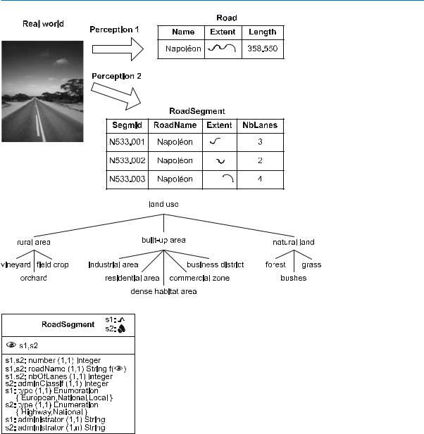
Modeling and Multiple Perceptions, Figure 12 Two different perceptions of the same reality, leading to different representations
Modeling and Multiple Perceptions, Figure 13 An example of a hierarchical domain
Modeling and Multiple Perceptions, Figure 14 An illustration of a birepresentation type, deÞned for perceptions s1 and s2
the diagrams, e. g., Fig. 14, the box identiÞed by the  icon deÞnes the set of perceptions for which this type is valid. Similarly, the speciÞcation of the relevant stamps is attached to each attribute and method deÞnition.
There are two complementary techniques to organize multiple representations. One solution is to build a single object type containing several representations, the knowledge of Òwhich representation belongs to which perceptionÓ being provided by the stamps of the properties of the type. Following this approach, in Fig. 14 the designer has
deÞned a single object type RoadSegment, grouping two representations, one for perception s1 and one for perception s2.
Definition 20: Multirepresentation Object/Relationship Types An object or relationship type is multirepresentation if at least one of its characteristics has at least two different representations. The characteristic may be at the schema level (e. g., an attribute with different deÞnitions) or at the instance level (i. e., different sets of instances or an instance with two different values).
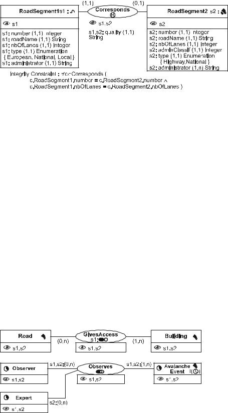
The alternative solution to organize multiple representations is to deÞne two separate object types, each one bearing the corresponding stamp(s) (cf. Fig. 15). The knowledge that the two representations describe the same entities is then conveyed by linking the object types with a relationship type that holds an interrepresentation semantics (indicated by the  icon). In the example of Fig. 15, the same real-world road segment is materialized in the database as two object instances, one in RoadSegment1 and one in RoadSegment2. Instances of the relationship type Corresponds tell which object instances represent the same road segment.
The actual representation of instances of multirepresentation object types changes from one perception to another.
|
|
|
|
|
Modeling and Multiple Perceptions |
689 |
|
|
|
|
|
|
|
|
|
|
|
|
|
|
|
|
|
|
|
|
|
|
|
|
|
|
|
|
|
|
|
|
|
|
|
Modeling and Multiple Perceptions, Figure 15 The
RoadSegment type (from Fig. 14) split into two monorepresentation object types and an interrepresentation relationship type
Consider the object type RoadSegment of Fig. 14. The spatial extent of the type is represented either as a surface (the more precise description, perception s2) or as a line (the less precise description, perception s1) depending on resolution. Furthermore, perception s1 needs the attributes number, roadName, numberOfLanes, type, and administrator (denoting the maintenance Þrm in charge). Perception s2 needs the attributes number, roadName, numberOfLanes, adminClassification, type, and administrator. While the road segment number and the number of lanes are the same for s1 and s2, the name of the road is different, although a string in both cases. For instance, the same road may have name ÒRN85Ó in perception s1 and name ÒRoute NapolŽonÓ in s2. We call this a perception-varying attribute (see below), identiÞed as such by the f( ) notation. The type attribute takes its values from predeÞned sets of values, the sets being different for s1 and s2. Several administrators for a road segment may be recorded for s2, while s1 records only one.
Definition 21: Perception-Varying Attribute An attribute is perception-varying if its value in an instance may change from one perception to another. A perception-vary- ing attribute is a function whose domain is the set of perceptions of the object (or relationship) type and whose range is the value domain deÞned for this attribute. These
attributes are the counterpart of space-varying and time- |
|
|||
varying attributes in the space and time modeling dimen- |
|
|||
sions. |
|
|
|
|
Stamps may also be speciÞed at the instance level. This |
|
|||
allows the deÞning of different subsets of instances that |
|
|||
are visible for different perceptions. For example, as the |
|
|||
object type RoadSegment in Fig. 14 has two stamps, it |
|
|||
is possible to deÞne instances that are only visible to s1, |
|
|||
instances that are only visible to s2, and instances that are |
|
|||
visible to both s1 and s2. |
|
|
|
|
|
|
M |
||
Relationship types |
can |
be |
in multirepresentation, |
|
like object types. Their structure (roles and associa- |
|
|||
tion/multiassociation |
kind) |
and |
semantics (e. g., topolo- |
|
gy, synchronization) may also have different deÞnitions |
|
|||
depending on the perception. Figure 16 shows an exam- |
|
|||
ple of different semantics, where the designer deÞned the relationship GivesAccess as (1) a topological adjacent relationship type for perception s1, and (2) a plain relationship without any peculiar semantics or constraint for perception s2.
A relationship type may have different roles for different perceptions. For example, Fig. 17 shows that an observation is perceived in s1 as a binary relationship between an observer and an avalanche event, while perception s2 sees the same observation as a ternary relationship, also involving the expert who has validated the observation.
Modeling and Multiple Perceptions, Figure 16 A relationship type with two different semantics: topological adjacency for s1 and plain relationship for s2
Modeling and Multiple Perceptions, Figure 17 A relationship type with a role specific to perception s2

690 Modeling Cycles in Geospatial Domains
Key Applications
Multirepresentation databases are an essential feature for all applications that need to provide different categories of users with different sets of data, organized in different ways, without imposing a single centralized model of the real world for the whole enterprise. Multirepresentation databases play a key role in guaranteeing and maintaining the consistency of a database with decentralized control and autonomy of updates from different user categories. Multiscale map production applications are one example of a domain where this feature is highly desirable. Management and analysis of municipal, regional, and statewide databases are other examples where the same geographic area is input to a variety of uses. Domain-oriented (e. g., environmental) interorganizational as well as international applications call for integrated databases that provide autonomous usage by the contributing organizations and countries.
Future Directions
Considering the large number of perceptions that some huge databases may have to support, an investigation into how perceptions may be organized and structured (as objects of interest per se) is planned.
Another direction for future research is adding complementary modeling dimensions to the MADS model, such as the multimedia dimension, the precision dimension (supporting, for example, fuzzy, imprecise, and approximate spatial and temporal features), and the trust or data quality dimension.
Finally, spatiotemporal and trajectory data warehousing represent wide-open research domains to develop efÞcient support for geographically based decision making.
6.Price, R., Ramamohanarao, K., Srinivasan, B.: Spatio-temporal Extensions to UniÞed Modeling Language. In: Proceedings of the Workshop on Spatio-temporal Data Models and Languages, IEEE DEXAÕ99 Workshop, Florence, Italy, 1Ð3 Sept 1999
7.BŽdard, Y., LarrivŽe, S., Proulx, M.J., Nadeau, M.: Modeling geospatial databases with plug-ins for visual languages: a pragmatic approach and the impacts of 16 years of research and experimentations on perceptory. In: Wang, S. et al. (eds.) ER Workshops, Shanghai, China. Lecture Notes in Computer Science, vol. 3289, pp. 17Ð30. Springer, Berlin, Heidelberg (2004)
8.David, B., Raynal, L., Schorter, G.: GeO2: Why objects in a geographical DBMS? In: Abel, D.J., Ooi, B.C. (eds.) Proceedings of the 3rd International Symposium on Advances in Spatial Databases, SSDÕ93, Singaporer, 23Ð25 June 1993. Lecture Notes in Computer Science, vol. 692, pp. 264Ð276. Springer Berlin, Heidelberg (1993)
9.BŽdard, Y., Bernier, ƒ.: Supporting multiple representations with spatial databases view management and the concept of VUEL. In: The Joint Workshop on Multi-Scale Representation of Spatial Data, ISPRS WG IV/3, ICA Commission. On Map Generalization, Ottawa, Canada, 7Ð8 July 2002
10.Parent, C., Spaccapietra, S., Zim‡nyi, E.: The MurMur Project: modeling and querying multi-represented spatio-tempo- ral databases. Inf. Syst. 31, 733Ð769 (2006)
11.Erwig, M., Schneider, M.: Spatio-temporal predicates. IEEE Trans. Knowledge Data Eng. 14, 881Ð901 (2002)
12.Weibel, R., Dutton, G.: Generalizing spatial data and dealing with multiple representations. In: Longley, P.A., Goodchild, M.F., Maguire, D.J., Rhind, D.W. (eds.) Geographical Information Systems: Principles, Techniques, Management and Applications, 2nd edn. vol. 1, pp. 125Ð155. Wiley, New York (1999)
14.Koubarakis, M. et al. (eds.): Spatio-temporal Databases: The Chorochronos Approach. Lecture Notes in Computer Science, vol. 2520. Springer, Berlin, Heidelberg (2003)
15.GŸting, R.H., Schneider, M.: Moving Objects Databases. Morgan Kaufmann, Amsterdam (2005)
16.Malinowski, E., Zim‡nyi, E.: Advanced data warehouse design: From conventional to spatial and temporal applications. Springer, Berlin, Heidelberg (2007, in press)
Modeling Cycles in Geospatial Domains
Cross References
JORGE CAMPOS
Modeling with ISO 191xx Standards Department of Exact Sciences,
Salvador University Ð UNIFACS, Salvador, Brazil
Recommended Reading
1.Chen, P.P.: The entity-relationship model: towards a uniÞed view of data. ACM Trans. Database Syst. 1, 9Ð36 (1976)
2.Rumbaugh, J., Jacobson, I., Booch, G.: The UniÞed Modeling Language, Reference Manual, 2nd edn. Addison-Wesley, Boston (2005)
Synonyms
Event, cyclic; Event, recurrent; Event, periodic
Definition
3.BŽdard, Y., Pageau, J., Caron, C.: Spatial data modeling: the
Modul-R formalism and CASE technology. In: Proceedings of In a geospatial context, cycles can be deÞned as regular-
the ISPRS Symposium, Washington, 1Ð14 Aug 1992
4.Tryfona, N., Jensen, C.S.: Conceptual Data Modeling for Spatiotemporal Application. GeoInformatica 3(3), 245-268 (1999)
5.Parent, C., Spaccapietra, S., Zim‡nyi, E.: Conceptual Modeling for Traditional and Spatio-temporal Applications: The MADS Approach. Springer, Berlin, Heidelberg (2006)
ly repeated phenomena or events. According to the distribution of this kind of happening over time, cycles can be classiÞed as strong periodic, near periodic, or intermittent. Strong periodicity refers to cycles in which the duration of every occurrence of the event is the same as