

prt%3A978-0-387-35973-1%2F16
.pdfModeling with Pictogrammic Languages |
721 |
Modeling with Pictogrammic Languages, Figure 4 Example of a single geometry pictogrammic expression (where each instance is represented by one line) and of an alternate geometry (where small buildings are represented by a point and large ones by a polygon) (Data from minist•re des Ressources naturelles et de la faune du QuŽbec)
Modeling with Pictogrammic Languages, Figure 5 Example of a multiple geometry pictogrammic expression, where at large scale (ex. 1:1000), buildings are represented by a polygon and at small scale (ex. 1:20 000), they are represented by a point, a line or nothing (Data from Research and Development Defence Canada and from minist•re des Ressources naturelles et de la faune du QuŽbec)
Using Pictogrammic Languages
for Spatio-temporal Database Modeling
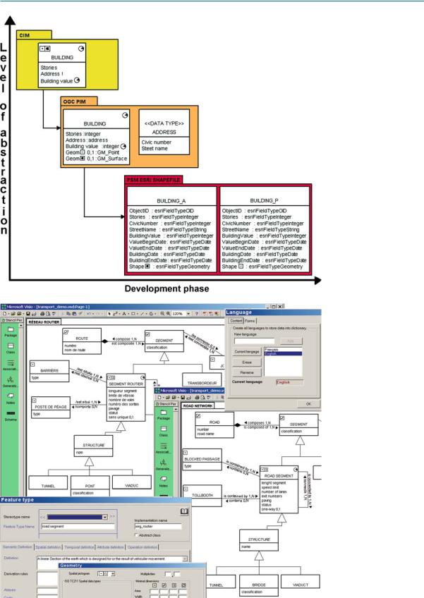
Modeling databases for GIS applications has always posed several challenges for system analysts, system developers as well as for their clients whose involvement into the development of such a project is not a familiar endeavor. Used with well-known modeling techniques, pictogrammic expressions help to meet these challenges [1,10,16,17] and are commonly used in different methods such as relational database design with UML (cf. the UML relational stereotypes in [15]). Extending CASE tools and modeling methods in such a way allows analysts and designers to work at a higher level of abstraction for the Þrst steps of a spatial database project. As presented in Fig. 6, once high-level models are completed (e. g. Perceptory CIM), they can be translated and enriched to give more technical models which are closer to implementation (e. g. OGC PIM, models by Brodeur and Badard in the chapter entitled ÒModeling with ISO 191xx StandardsÓ) and Þnally
highly technical models which speciÞc to one implementation on one platform (e. g. ESRI ShapeÞles PSM). Such multi-level approach is typical of good software engineering methods as exempliÞed in Fig. 6 and by the following landmark methods:
¥The Object Management Group (OMG) Model-Driven Architecture (MDA) which has three levels of models: Computation Independent Model (CIM), Platform Independent Model (PIM) and Platform SpeciÞc Model (PSM);
¥Zachman Framework [12,18] which has a business or enterprise model, a system model and a technology model (also called semantic, logical and physical models);
¥Rational UniÞed Process (RUP) which has a domain model, an analysis model, a design model and an imple-
mentation model. |
|
|
Since the pictograms are aimed at facilitating modeling |
|
|
by being closer to human language than typical model- |
|
|
ing artefacts, they are primarily used in high-level models. |
|
|
Regarding the MDA method, pictogrammic expressions |
|
|
are more widely used for CIM than for PIM and PSM: |
|
|
¥ CIM: ÒA computation independent model is a view of |
|
|
M |
||
a system from the computation independent viewpoint. |
||
A CIM does not show details of the structure of sys- |
|
|
|
||
tems. A CIM is sometimes called a domain model and |
|
|
a vocabulary that is familiar to the practitioners of the |
|
|
domain in question is used in its speciÞcation.Ó[13] |
|
¥PIM: ÒA platform independent model is a view of a system from the platform independent viewpoint. A PIM exhibits a speciÞed degree of platform independence so as to be suitable for use with a number of different platforms of similar type.Ó [13]
¥PSM: ÒA platform specific model is a view of a system from the platform speciÞc viewpoint. A PSM combines the speciÞcations in the PIM with the details that specify how that system uses a particular type of plat-
form.Ó [13]
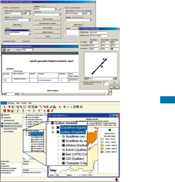
Furthermore, since pictograms are not tied to a speciÞc natural language, they facilitate the translation of database models. For example, in Canada, several schemas and repositories are available in English and French. Figure 7 shows such French and English schemas that are synchronized thru the same repository and pictograms. The use of formal ISO-19110 labels (in blue) further facilitates communication while the use of pictograms facilitates automatic GIS code generation and bilingual reporting.
At the CIM level, pictogrammic expressions are intuitive and independent of domain ontologies and technology-ori- ented standards. No technology artefacts nor standardization elements must appear unless they are useful and intuitive. When the CIM is well deÞned, it can be translated
722 Modeling with Pictogrammic Languages
Modeling with Pictogrammic Languages, Figure 6
Examples of CIM, PIM and PSM levels of abstraction of the MDA method for a same application, where the information encapsulated in the higher levels using pictograms is expanded in the lower levels
Modeling with Pictogrammic Languages, Figure 7
Example of common pictograms in a French and an English CIM synchronized for a same spa- tio-temporal database using Perceptory multi-standard and multi-language capabilities
Modeling with Pictogrammic Languages |
723 |
Modeling with Pictogrammic Languages, Figure 8
Examples of pictogrammic expressions to deÞne topological constraints between two object classes (upper left), to print them in a report (lower left) and to describe them in an extended ISO e-related 3 × 3 matrix
M
Modeling with Pictogrammic Languages, Figure 9
JMap SOLAP interface using pictogrammic expressions
and enriched to produce lower-level models semi-automat- ically. Then, technology-oriented artefacts and standardbased elements replace the pictogrammic expressions. For example, in Fig. 6, the CIM evolves in a PIM where the geometry is expressed according to ISO/OGC. Then, the PSM shows the structure of two shapeÞles needed to implement Building Points and Building Areas.
In addition to hiding the technical complexities of GIS and Universal server database engines, using pictogrammic expressions also hides the intricacies of international standards such as ISO/TC-211 and OGC. For example, ISO jargon doesnÕt express directly all possible geometries (ex. alternate and facultative geometries) and they are not cognitively compatible with clientsÕ conceptual view who

724 Modeling with Pictogrammic Languages
assumes a topologically consistent world (ex. GMPoint vs TPNode, GMCurve vs TPEdge, GMSurface vs TPFace, Aggregate vs Multi).
Using Pictogrammic Expressions
to Define Spatial Integrity Constraints
Spatial integrity constraints can also be deÞned efÞciently with pictogrammic expressions. For example, in Fig. 8, the upper window shows a user interface for the deÞnition of spatial integrity constraints between two object classes, with or without considerations to speciÞc attribute values. The lower window shows a report showing the deÞned spatial integrity constraints. The last window shows an example of using pictogrammic expressions in a 3 × 3 e-relate matrix.
Additional Usages of Pictogrammic Expressions:
Software User Interfaces, Reports and Semantic
Proximity Analysis
Pictogrammic expressions are regularly used in a text to express the spatiality and temporality of objects. They have been used in reports, data dictionaries and data acquisition speciÞcations. They were also used for semantic proximity analysis [9] and integrated in a commercial package (JMap SOLAP, Fig. 9).
Future Directions
Over the last two decades, different pictogrammic languages have emerged to improve the efÞciency of systems analysts and to improve the quality of spatial database design. The language presented in this chapter was the Þrst such language and has become the most widely used one, not only within Perceptory but also in other CASE tools and in diverse applications. It uses a downloadable font (http://sirs.scg.ulaval.ca/YvanBedard/ english/others.asp). Such languages will likely evolve in two major directions. First, they will accommodate the most recent spatial database trends, that is spatial datacube structures for data warehousing and SOLAP applications. Second, as they can be translated into ISO and OGC primitives [8], ofÞcial adoption of such a language should be put forward to improve interoperability between spatial application database schemas, between ontologies and between other documents.
Cross References
Modeling and Multiple Perceptions
Modeling with Enriched Model Driven Architecture
Modeling with a UML ProÞle
Modeling with ISO 191xx Standards
Spatio-temporal Database Modeling with an Extended Entity-Relationship Model
Recommended Reading
1.BŽdard, Y., LarrivŽe, S., Proulx, M.-J., Nadeau, M.: Modeling Geospatial Databases with Plug-Ins for Visual Languages: A Pragmatic Approach and the Impacts of 16 Years of Research and Experimentations on Perceptory. In: Wang, S. et al. (eds.): Conceptual Modeling for Advanced Application Domains. Lecture Notes in Computer Science, Vol. 3289, pp. 17Ð30. SpringerVerlag, Berlin/Heidelberg (2004)
2.BŽdard, Y., Proulx, M.-J., LarrivŽe, S., Bernier, E.: Model-
ing Multiple Representations into Spatial Data Warehouses: A UML-based Approach. ISPRS WG IV/3, Ottawa, Canada, July 8thÐ12th, p. 7 (2002)
3.BŽdard, Y.: Visual Modeling of Spatial Database, Towards Spatial PVL and UML. Geomatica 53(2), 169Ð185 (1999)
4. BŽdard, Y., Caron, C., Maamar, Z., Moulin, B., Valli•re, D.: Adapting Data Model for the Design of Spatio-Temporal Database. Comput., Environ. Urban Syst. 20(l), 19Ð41 (1996)
5.BŽdard, Y., Pageau, J., Caron, C.: Spatial Data Modeling: The Modul-R Formalism and CASE Technology. ISPRS Symposium, Washington DC, USA, August 1stÐ14th (1992)
6.BŽdard, Y., Paquette, F.: Extending Entity/Relationship Formalism for Spatial Information Systems. AUTO-CARTO 9, 9th International Symposium on Automated Cartography, ASPRSACSM, Baltimore, USA, pp. 818Ð827, April 2ndÐ7th (1989)
7.BŽdard, Y., LarrivŽe, S.: DŽveloppement des syst•mes dÕinformation ˆ rŽfŽrence spatiale: vers lÕutilisation dÕateliers de gŽnie logiciel. CISM Journal ACSGC, Canadian Institute of Geomatics, Canada, 46(4), 423Ð433 (1992)
8.Brodeur, J., BŽdard, Y., Proulx, M.-J.: Modeling Geospatial Application Database using UML-Based Repositories Aligned with International Standards in Geomatics. ACM-GIS, Washington DC, USA, 36Ð46, November 10thÐ11th (2000)
9.Brodeur, J., BŽdard, Y., Edwards, G., Moulin, B.: Revisiting the Concept of Geospatial Data Interoperability within the Scope of Human Communication Processes. Transactions in GIS 7(2), 243Ð265 (2003)
10.Filho, J.L., Sodre, V.D.F., Daltio, J., Rodrigues Junior, M.F., Vilela, V.: A CASE Tool for Geographic Database Design Supporting Analysis Patterns. Lecture Notes in Computer Science, vol. 3289, pp. 43Ð54. Springer-Verlag, Berlin/Heidelberg (2004)
11.Fowler, M.: UML 2.0, p. 165. Campus Press, Pearson Education, Paris (2004)
12.Frankel, D.S., Harmon, P., Mukerji, J., Odell, J., Owen, M., Rivitt, P., Rosen, M., Soley, R.: The Zachman Framework and the OMGÕs Model Driven Architecture. Business Process Trends, Whitepaper (2003)
13.Miller, J., Mukerji, J.: MDA Guide Version 1.0. In: Miller, J., Mukerji, J. (eds.), OMG Document: omg/2003-05-01. http:// www.omg.org/mda/mda_Þles/MDA_Guide_Version1-0.pdf (2003)
14.Miralles, A.: IngŽnierie des mod•les pour les applications environnementales. Ph.D. Thesis, UniversitŽ des Sciences et Techniques du Languedoc, p. 338. DŽpartement dÕinformatique, Montpellier, France (2006)
15.Naiburg, E.J., Maksimchuk, R.A.: UML for Database Design. Addison-Wesley, p. 300 (2001)
16.Pantazis, D., Donnay, J.P.: La conception SIG: mŽthode et formalisme, p. 343. Herm•s, Paris (1996)

Movement 725
17.Parent, C., Spaccapietra, S., Zim‡nyi, E.: Conceptual Modeling for Traditional and Spatio-Temporal Applications: The MADS Approach, p. 466. Springer, Berlin/Heidelberg (2006)
and wij is the element of the spatial weights matrix for locations i and j, deÞned as 1 if location i is contiguous to location j and 0 otherwise. Other more complicated deÞni-
18.Sowa, J.F., Zachman, J.A.: Extending and Formalizing the
Framework for Information Systems Architecture. IBM Syst. J. tions of spatial weights matrices allow for the computation
31(3). IBM Publication G321Ð5488 (1992)
19.Tryfona, N., Price, R., Jensen, C.S.: Conceptual Models for Spa- tio-Temporal Applications. In Spatiotemporal Databases: The CHOROCHRONOS approach, Lecture Notes in Computer Science, vol. 2520, Chapter 3. Springer-Verlag, Berlin/Heidelberg (2003)
Modifiable Areal Unit Problem
Error Propagation in Spatial Prediction
Monitoring
Data Collection, Reliable Real-Time
of the MoranÕs I at various levels of proximity or distance.
Main Text
MoranÕs I is one of the oldest indicators of spatial autocorrelation and is still a widely accepted measure for determining spatial autocorrelation. It is used to estimate the strength of interdependence between observations of the variable of interest as a function of the distance by comparing the value of xi at location i with the value xj at all other locations (j = i). MoranÕs I varies from −1 to 1. Positive signage represents positive spatial autocorrelation, while the negative signage represents negative spatial autocorrelation. The MoranÕs I will approach zero for a large sample size when the variable values are randomly distributed and independent in space.
Monte Carlo Simulation
Uncertain Environmental Variables in GIS Cross References
Autocorrelation, Spatial
M
Moran Coefficient
MoranÕs I
Moran’s Index
Moran’s I
XIAOBO ZHOU, HENRY LIN
Department of Crop and Soil Sciences, The Pennsylvania State University, University Park, PA, USA
Synonyms
MoranÕs index; Moran coefÞcient
Definition
MoranÕs I, based on cross-products, measures value association and is calculated for n observations on a variable x at locations i, j as
wij(xi − x¯)(xj − x¯)
I = |
i j=i |
|
|
. |
|
S2 |
wij |
||
|
|
i |
j=i |
|
Where xi denotes the observed value at location i, x¯ is the mean of the x variable over the n locations,
S2 |
1 |
(xi − x¯)2 , |
|
= |
|
||
n |
|||
|
|
|
i |
MoranÕs I
Motion Patterns
Movement Patterns in Spatio-temporal Data
Motion Tracking
Moving Object Uncertainty
Moved Planning Process
Participatory Planning and GIS
Movement
Temporal GIS and Applications
726 Movement Patterns in Spatio-temporal Data
Movement Patterns
in Spatio-temporal Data
JOACHIM GUDMUNDSSON1, PATRICK LAUBE2,
THOMAS WOLLE1
1NICTA, Sydney, NSW, Australia
2Department of Geomatics, University of Melbourne, Melbourne, VIC, Australia
Synonyms
Motion patterns; Trajectory patterns; Exploratory data analysis; Flocking; Converging; Collocation, spatio-tem- poral; Indexing trajectories; TPR-trees; R-tree, multiversion; Indexing, parametric space; Indexing, native space; Association rules, spatio-temporal; Pattern, moving cluster; Pattern, periodic; Pattern, leadership; Pattern, ßock; Pattern, encounter
Definition
Spatio-temporal data is any information relating space and time. This entry speciÞcally considers data involving point objects moving over time. The terms entity and trajectory will refer to such a point object and the representation of its movement, respectively. Movement patterns in such data refer to (salient) events and episodes expressed by a set of entities.
In the case of moving animals, movement patterns can be viewed as the spatio-temporal expression of behaviors, as for example in ßocking sheep or birds assembling for the
seasonal migration. In a transportation context, a movement pattern could be a trafÞc jam.
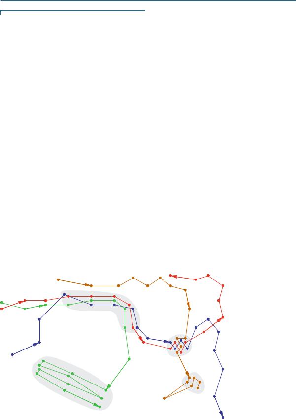
Only formalized patterns are detectable by algorithms. Hence, movement patterns are modeled as any arrangement of subtrajectories that can be sufÞciently deÞned and formalized, see for example the patterns illustrated in Fig. 1. A pattern usually involves a certain number of entities. Furthermore a pattern starts and ends at certain times (temporal footprint), and it might be restricted to a subset of space (spatial footprint).
Historical Background
The analysis of movement patterns in Spatio-temporal data is for two main reasons a relatively young and little developed research Þeld. First, emerging from static cartography, geographical information science and theory struggled for a long time with the admittedly substantial challenges of handling dynamics. For many years, occasional changes in a cadastral map were challenging enough, not to mention the constant change of location as is needed for modeling movement.
Second, only in recent years has the technological advancement in tracking technology reached a level that allowed the seamless tracking of individuals needed for the analysis of movement patterns. For many years, the tracking of movement entities has been a very cumbersome and costly undertaking. Hence, movement patterns could only be addressed for single individuals or very small groups. HŠgerstrandÕs time geography [10] may serve as a starting point of a whole branch of geographical information science representing individual trajectories in 3D. The two
flock with |
|
three entities |
meeting |
|
place |
frequent |
location |
periodic pattern
Movement Patterns in Spa- tio-temporal Data, Figure 1
Illustrating the trajectories of four entities moving over 20 time steps. The following patterns are highlighted: a flock of three entities over Þve time-steps,
a periodic pattern where an entity shows the same Spatiotemporal pattern with some periodicity, a meeting place where three entities meet for four time steps, and Þnally, a frequently visited location which is a region where a single entity spends
a lot of time
Movement Patterns in Spatio-temporal Data |
727 |
GIScience |
Database |
Management |
Computational |
Geometry |
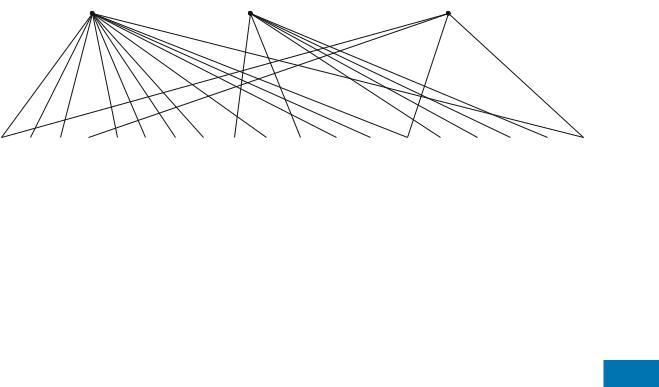
[1] [2] [3] [4] [5] [6] [7] [8] [9] [10] [11] [12] [13] [14] [15] [16] [17] [18] [19]
Movement Patterns in Spatio-temporal Data, Figure 2 Access guide to the references in the recommended reading section below
spatial dimensions combined with an orthogonal temporal axis proved to be a very powerful concept for exploring various kinds of spatio-temporal relationships, including movement patterns.
With GPS and various other tracking technologies movement pattern research entered a new era, stepping from Ôthread trailingÕ and Ômark and recaptureÕ approaches to low cost, almost continuous capture of individual trajectories with possibly sub-second sampling rates. Within a few years the situation completely reversed from a notorious data deÞcit to almost a data overkill, with a lack of suited analytical concepts coping with the sudden surge of movement data. Consequently, the huge potential of analyzing movement in spatio-temporal data has recently attracted the interest of many research Þelds, both in theory and application, as is outlined in the next two sections.
Scientific Fundamentals
Assume that the entities in Fig. 1 are sheep on a pasture and that they are observed by a geographer, a database expert and a computational geometer. Even though all three experts see the very same sheep, they may all perceive totally different things. The geographer might interpolate a sheep density surface of the pasture. For the database expert in contrast, each sheep may represent a leaf in a dynamic tree optimized for fast queries. Finally, the computational geometer might triangulate the sheep locations in order to detect a ßocking pattern. Even though the sheep will not care, their grazing challenges various research Þelds handling spatio-temporal data. The following overview bundles the different perspectives addressing movement patterns into the three sections exploration, indexing and data mining. See Fig. 2 for a comprehensible access guide to recommended reading.
GIScience: Exploratory Data Analysis
and Visualization
In GIScience the term ÔpatternÕ is used in various contexts and meanings when addressing movement. However, as a common denominator, movement patterns are general-
ly conceptualized as salient movement events or episodes |
|
|||
in the geospatial representation of moving entities. Given |
|
|||
GIScienceÕs legacy in cartography, it is not surprising that |
|
|||
movement patterns are often addressed by a combination |
|
|||
of geovisualisation and exploration. Exploratory analysis |
|
|||
approaches combine the speed and patience of comput- |
|
|||
ers with the excellent capability of humans to detect the |
|
|||
expected and discover the unexpected given an appropri- |
|
|||
ate graphical representation. |
|
|
|
|
Salient movement patterns may emerge from (i) two- |
|
|||
dimensional maps of |
Þxes aligned |
in |
trajectories, |
M |
(ii) movie-like animated maps or even (iii) three-dimen- |
||||
sional representations of |
movement, if |
time |
is used as |
|
a third, orthogonal axis.
(i)Basic movement patterns are obvious from simple plotting of movement trajectories on a two-dimensional map. Trajectories bundled in narrow, directed bottlenecks represent often used corridors. Less focused trajectory footprints represent more arbitrary movement, such as in grazing animals or visitors at a sports event strolling around a stadium. The application of GUS analysis tools on points and lines representing moving entities has proven to be a very effective approach. For example, GIS tools for generalization, interpolation and surface generation may be applied to support the detection of movement patterns in trajectory data. Brillinger et al. [5] use a regularly sampled vector Þeld to illustrate the overall picture of animals moving in their habitat, with each vector coding in orientation and size for mean azimuth and mean speed at that very location. Dykes and Mountain [8] use a continuous density surface and a ÔspotlightÕ metaphor for the detection of activity patterns. Again, common GIS tools such as algorithms initially designed for the analysis of digital terrain models can easily be adopted for the search for salient movement patterns, for instance to identify ÔpeaksÕ of frequent visitation and ÔridgesÕ of busy corridors [8].
(ii)Animation is suited to uncover speciÞc movement behaviors of individuals and groups. Animating moving entities with a constant moving time window in the socalled dynamic view uncovers speed patterns of individ-

728 Movement Patterns in Spatio-temporal Data
uals [2,8]. Flocking or converging are more complex patterns of coordination in groups. Such group patterns are very striking when animating even large numbers or individuals in a movie-like animation.
(iii) The extension of a two-dimensional map with a third orthogonal time axis produces a very powerful tool for uncovering movement patterns. Such ideas go back to HŠgerstrandÕs time geography [10] and have often been adopted in present day geocomputation [12]. In the specific geometry in such a three-dimensional space-time aquarium episodes of immobility and certain speed behaviors produce distinctive patterns of vertical and inclined time lines, respectively. Furthermore, patterns of spatio-tempo- ral collocation can be identiÞed from vertical bottleneck structures in sets of time lines [12].
Indexing Spatio-temporal Trajectories
In the database community considerable research has been focusing on spatial and temporal databases. Research in the spatio-temporal area in many ways started with the dissertations by Lorentzos [15] in 1988 and Langran [13] in 1989. Not surprisingly research has mainly focused on indexing databases so that basic queries concerning the data can be answered efÞciently. The most common queries considered in the literature are variants of nearest neighbor queries and range searching queries. For example:
¥Spatio-temporal range query, e. g. ÔReport all entities that visited region S during the time interval [t1,t2].Õ
¥ |
Spatial nearest |
neighbors |
given |
a |
time |
interval, |
|
e. g. ÔReport the entity closest to point p at time t.Õ |
|||||
¥ |
Temporal nearest |
neighbors |
given |
a |
spatial |
region, |
e. g. ÔReport the Þrst entity visiting region S.Õ
In general one can classify indexing methods used for spa- tio-temporal data into Parametric Space Indexing methods (PSI) and Native Space Indexing methods (NSI). The PSI method uses the parametric space deÞned by the movement parameters, and is an efÞcient approach especially for predictive queries. A typical approach, described by Sÿaltenis et al. [17] is to represent movement deÞned by its velocity and projected location along each spatial dimension at a global time reference. The parametric space is then indexed by a new index structure referred to as the TPR-tree (Time Parametrized R-tree). The TPR-tree is a balanced, multi-way tree with the structure of an R-tree. Entries in leaf nodes are pairs of the position of a moving point and a pointer to the moving point, and entries in internal nodes are pairs of a pointer to a subtree and a rectangle that bounds the positions of all moving points or other bounding rectangles in that subtree. The position of a moving point is represented by a reference position and
a corresponding velocity vector. To bound a group of d- dimensional moving points, d-dimensional bounding rectangles are used that are also time parametrized, i. e. their coordinates are functions of time. A time-parametrized bounding rectangle bounds all enclosed points or rectangles at all times not earlier than the current time. The search algorithm for a range query also performs computation on the native space by checking the overlap between the range of the query and the trapezoid representation of the node.
The NSI methods represent movement in d dimensions as a sequence of line segments in d + 1 dimensions, using time as an additional dimension, see for example the work by Hadjieleftheriou et al. [9]. A common approach is to use a multi-dimensional spatial access method like the R- tree. An R-tree would approximate the whole spatio-tem- poral evolution of an entity with one Minimum Bounding Region (MBR) that tightly encloses all the locations occupied by the entity during its lifetime. An improvement for indexing movement trajectories is to use a multi version index, like the Multi Version R-tree (MVR-tree), also known as a persistent R-tree. This index stores all the past states of the data evolution and allows updates to the most recent state. The MVR-tree divides long-lived entities into smaller intervals by introducing a number of entity copies. A query is directed to the exact state acquired by the structure at the time that the query refers to; hence, the cost of answering the query is proportional to the number of entities that the structure contained at that time.
Algorithms and Data Mining
In the previous section different indexing approaches were discussed. This section will focus on mining trajectories for spatio-temporal patterns. This has mainly been done using algorithmic or data mining approaches.
The most popular tools used in the data mining community for spatio-temporal problems has been association rule mining (ARM) and various types of clustering. Association rule mining seeks to discover associations among transactions within relational databases. An association rule is of the form X Y where X (antecedents) and Y (consequents) are disjoint conjunctions of attribute-value pairs. ARM uses the concept of confidence and support. The conÞdence of the rule is the conditional probability of Y given X, and the support of the rule is the prior probability of X and Y.
The probability is usually the observed frequency in the data set. Now the ARM problem can be stated as follows. Given a database of transactions, a minimal conÞdence threshold and a minimal support threshold, Þnd all asso-

Movement Patterns in Spatio-temporal Data |
729 |
ciation rules whose conÞdence and support are above the corresponding thresholds.
Chawla and Verhein [18] deÞned spatio-temporal association rules (STARs) that describe how entities move between regions over time. They assume that space is partitioned into regions, which may be of any size and shape. The aim is to Þnd interesting regions and rules that predict how entities will move through the regions. A region is interesting when a large number of entities leaves (sink), a large number of entities enters (source) or a large number of entities enters and leaves (thoroughfare).
A STAR (ri,T1,q) (rj,T2) denotes a rule where entities in a region ri satisfying condition q during time interval T1 will appear in region rj during time interval T2. The support of a rule δ is the number, or ratio, of entities that follow the rule. The spatial support takes the size of the involved regions into consideration. That is, a rule with support s involving a small region will have a larger spatial support than a rule with support s involving a larger region. Finally, the conÞdence of a rule δ is the conditional probability that the consequent is true given that the antecedent is true. By traversing all the trajectories all possible movements between regions can be modeled as a rule, with a spatial support and conÞdence. The rules are then combined into longer time intervals and more complicated movement patterns.
Some of the most interesting spatio-temporal patterns are periodic patterns, e. g. yearly migration patterns or daily commuting patterns. Mamoulis et al. [16] considered the special case when the period is given in advance. They partition space into a set of regions which allows them to deÞne a pattern P as a τ -length sequence of the form r0, r1, . . . , rτ −1, where ri is a spatial region or the special character *, indicating the whole spatial universe. If the entity follows the pattern enough times, the pattern is said to be frequent. However, this deÞnition imposes no control over the density of the regions, i. e. if the regions are too large then the pattern may always be frequent. Therefore an additional constraint is added, namely that the points of each subtrajectory should form a cluster inside the spatial region.
Kalnis et al. [11] deÞne and compute moving clusters where entities might leave and join during the existence of a moving cluster. For each Þxed discrete time-step ti they use standard clustering algorithms to Þnd clusters with a minimum number of entities and a minimum density. Then they compare any cluster c found for ti with any (moving) cluster c found for time-step ti-1. If c and c have enough entities in common, which is formally speciÞed by a threshold value, then c can be extended by c, which results in a moving cluster. They propose several ideas to increase the speed of their method, e. g. by avoiding redun-
dant cluster comparisons, or approximating moving clusters instead of giving exact solutions, and they experimentally analyze their performance.
In 2004 Laube et al. [14] deÞned a collection of spa- tio-temporal patterns based on direction of movement and location, e. g. ßock, leadership, convergence and encounter, and they gave algorithms to compute them efÞciently. As a result there were several subsequent articles studying the discovery of these patterns. Benkert et al. [4] modiÞed the original deÞnition of a ßock to be a set of entities moving close together during a time interval. Note that in this deÞnition the entities involved in the ßock must be the same during the whole time interval, in contrast to the moving cluster deÞnition by Kalnis et al. [11]. Benkert et al. [4] observed that a ßock of m entities moving together during k time steps corresponds to a cluster of size m in 2k dimensional space. Thus the problem can be restated as clustering in high dimensional space. To handle high dimensional space one can use well-known dimensionality reduction techniques. There are several decision versions of the problem that have been shown to be NP-hard, for example deciding if there exists a ßock of a certain size, or of a certain duration. The special case when the ßock is
stationary is often called a meeting pattern. M Andersson et al. [1] gave a more generic deÞnition of the pattern leadership and discussed how such leadership pat-
terns can be computed from a group of moving entities. The proposed deÞnition is based on behavioral patterns discussed in the behavioral ecology literature. The idea is to deÞne a leader as an entity that (1) does not follow anyone else, (2) is followed by a set of entities and (3) this behavior should continue for a duration of time. Given these rules all leadership patterns can be efÞciently computed.
Be it exploratory analysis approaches, indexing techniques or data mining algorithms, all effort put in theory ultimately leads to more advanced ways of inferring high level process knowledge from low level tracking data. The following section will illustrate a wide range of Þelds where such fundamentals underlie various powerful applications.
Key Applications
Animal Behavior
The observation of behavioral patterns is crucial to animal behavior science. So far, individual and group patterns are rather directly observed than derived from tracking data. However, there are more and more projects that collect animal movement by equipping them with GPSGSM collars. For instance, since 2003 the positions of 25 elks in Sweden are obtained every 30 minutes. Other researchers attached small GPS loggers to racing pigeons

730 Movement Patterns in Spatio-temporal Data
and tracked their positions every second during a pigeonÕs journey. It is even possible to track the positions of insects, e. g. butterßies or bees, however most of the times nonGPS based technologies are used that allow for very small and light sensors or transponders. Analyzing movement patterns of animals can help to understand their behavior in many different aspects. Scientists can learn about places that are popular for individual animals, or spots that are frequented by many animals. It is possible to investigate social interactions, ultimately revealing the social structure within a group of animals. A major focus lies on the investigation of leading and following behavior in socially interacting animals, such as in a ßock of sheep or a pack of wolves [7]. On a larger scale, animal movement data reßects very well the seasonal or permanent migration behavior. In the animation industry, software agents implement movement patterns in order to realistically mimic the behavior of animal groups. Most prominent is the ßocking model implemented in NetLogo which mimics the ßocking of birds [19].
Human Movement
Movement data of people can be collected and used in several ways. For instance, using mobile phones that communicate with a base station is one way to gather data about the approximate locations of people. TrafÞc-monitoring devices such as cameras can deliver data on the movement of vehicles. With the technological advancement of mobile and position aware devices, one could expect that tracking data will be increasingly collectable. Although tracking data of people might be available in principle, ethical and privacy aspects need to be taken into consideration before gathering and using this data [6]. Nonetheless, if the data is available, it could be used for urban planning, e. g. to plan where to build new roads or where to extend public transport.
The detection of movement patterns can furthermore be used to optimize the design of location-based-services (LBS). The services offered to a moving user could not only be dependent on the actual position, but also on the estimated current activity, which may be derived from a detected movement pattern.
Traffic Management
Movement patterns are used for trafÞc management in order to detect undesirable or even dangerous constellations of moving entities, such as trafÞc jams or airplane course conßicts. TrafÞc management applications may require basic Moving Object Database queries, but also more sophisticated movement patterns involving not
just location but also speed, movement direction and other activity parameters.
Surveillance and Security
Surveillance and intelligence services might have access to more detailed data sets capturing the movement of people, e. g. coordinates from mobile phones or credit card usage, video surveillance camera footage or maybe even GPS data. Apart from analyzing the movement data of a suspect to help prevent further crime, it is an important task to analyze the entire data set to identify suspicious behavior in the Þrst place. This leads to deÞne Ônormal behaviorÕ and then search the data for any outliers, i. e. entities that do not show normal behavior. Some speciÞc activities and the corresponding movement patterns of the involved moving entities express predeÞned signatures that can be automatically detected in spatio-temporal or footage data. One example is that Þshing boats in the sea around Australia have to report their location in Þxed intervals. This is important for the coast guards in case of an emergency, but the data can also be used to identify illegal Þshing in certain areas. Another example is that a car thief is expected to move in a very characteristic and hence detectable way across a surveilled car park. Movement patterns have furthermore attracted huge interests in the Þeld of spatial intelligence and disaster management. Batty et al. [3] investigated local pedestrian movement in the context of disaster evacuation where movement patterns such as congestion or crowding are key safety issues.
Military and Battlefield
The digital battleÞeld is an important application of moving object databases. Whereas real-time location data of friendly troops is easily accessible, the enemyÕs location may be obtained from reconnaissance planes with only little time lag. Moving object databases not only allow the dynamic updating of location and status of tanks, airplanes and soldiers, but also answering spatio-temporal queries and detecting complex movement patterns. Digital battleÞeld applications answer spatio-temporal range queries like ÔReport all friendly tanks that are currently in region S.Õ A more complex movement pattern in a digital battleÞeld context would be the identiÞcation of the convergence area where the enemy is currently concentrating his troops.
Sports Scene Analysis
Advancements in many different areas in technology are also inßuencing professional sports. For example, some of the major tennis tournaments provide three-dimension- al reconstructions of every single point played, tracking the players and the balls. It is furthermore known