

prt%3A978-0-387-35973-1%2F16
.pdfMLPQ Spatial Constraint Database System |
661 |
Cross References
Indexing Spatial Constraint Databases
Plane Sweep Algorithm
Recommended Reading
1.Shekhar, S., Chawla, S.: Spatial Databases, A Tour, Pearson Education, Inc., New Jersey, USA (2003) ISBN 0-13-017480-7
Minimum Bounding Rectangles
Oracle Spatial, Geometries
Definition
The MLPQ system [1,2,3] is a spatial constraint database system developed at the University of Nebraska-Lincoln. The name of the system is an acronym for Management of Linear Programming Queries. The special feature of the MLPQ system is that it can run both SQL and Datalog queries on spatial constraint databases with linear inequality constraints. The MLPQ system is applied in the area of geographic information systems, moving objects databases and operations research. The MLPQ system has an advanced graphical user interface that displays maps and animates changes over time. Using a library of special routines, MLPQ databases can be easily made webaccessible.
Minimum Orthogonal Bounding Rectangle
Minimum Bounding Rectangle
Mining Collocation Patterns
Co-location Patterns, Algorithms
Mining Sequential Patterns from Spatio-Temporal Databases
Sequential Patterns, Spatio-temporal
Mining Spatial Association Patterns
Co-location Patterns, Algorithms
Mining Spatio-Temporal Datasets
Trajectories, Discovering Similar
MLPQ Spatial Constraint
Database System
PETER REVESZ
Department of Computer Science and Engineering, University of Nebraska-Lincoln, Lincoln, NE, USA
Synonyms
Management of linear programming queries; MLPQ system
Main Text
The MLPQ system accepts input textÞles speciÞed as a set of constraint tuples or facts. Each atomic constraint must written in a way that all variables are on the left hand side of the >= comparison operator meaning Ògreater than or equal.Ó For example, the Lincoln town area can be repre-
sented as follows.
M
begin %Lincoln-area%
Lincoln (id, x, y, t) :- id = 1, y − x >= 8, y >= 14, x >= 2, −y >= − 18,
−y − z >= −24.
Lincoln (id, x, y, t) :- id = 2, x − y >= −8, 0.5 x − y >= −12,
−y >= −18, x >= −14, y >= 8, 3x + y >= 32.
end %Lincoln-area%
The MLPQ allows browsing of the directory of input data Þles. Once an input dataÞle is selected, then the system immediately displays it on the computer screen. For queries and advanced visualization tools a number of graphical icons are available. For example, when clicking on the icon that contains the letters SQL a dialog box will be called. The dialog box allows selection of the type of SQL query that the user would like to enter. The types available are basic, aggregate, nested, set, and recursive SQL queries. Suppose one clicks on AGGREGATE. The a new dialog box will prompt for all parts of an aggregate SQL query, including the part that creates an output Þle with a speciÞc name as the result of executing the query. For example, one can enter either of the SQL queries that one saw in the entry on Spatial Constraint Databases. When the SQL query is executed and the output relation is created, it is shown on the left side of the computer screen. Clicking on the name of the output relation prompts MLPQ to display it as a spatial constraint database table and/or as a map if that is possible. MLPQ requires each constraint tuple to have an id as its Þrst Þeld (this

662 MLPQ System
helps internal storage and indexing); however, any number of spatiotemporal and non-spatiotemporal Þelds can follow the id Þeld. If there are more than two spatial Þelds, then the projections to the Þrst two spatial Þelds (assumed to be the second and third Þelds) are displayed only. To visualize moving objects with a growing or shrinking spatial area, special animation algorithms need to be called. The system is available free from the authorÕs webpage at cse.unl.edu/~revesz.
Cross References
Constraint Database Queries
Indexing Spatial Constraint Databases
Visualization of Spatial Constraint Databases
Recommended Reading
1.Kanjamala, P., Revesz, P., Wang, Y.: MLPQ/GIS: A GIS using linear constraint databases. Proc. 9th COMAD International Conference on Management of Data, pp. 389Ð393. McGraw-Hill, New Delhi (1998)
2.Revesz, P., Chen, R., Kanjamala, P., Li, Y., Liu, Y., Wang, Y.: The MLPQ/GIS Constraint Database System. In: Proc. ACM SIGMOD International Conference on Management of Data. ACM Press, New York (2000)
3.Revesz, P., Li, Y.: MLPQ: A linear constraint database system with aggregate operators. In: Proc. 1st International Database Engineering and Applications Symposium, pp. 132Ð7. IEEE Press, Washington (1997)
MLPQ System
MLPQ Spatial Constraint Database System
Mobile Maps
Web Mapping and Web Cartography
Mobile Object Indexing
GEORGE KOLLIOS1, VASSILIS TSOTRAS2,
DIMITRIOS GUNOPULOS2
1Department of Computer Science, Boston University, Boston, MA, USA
2Department of Computer Science and Engineering, University of California-Riverside, Riverside, CA, USA
Synonyms
Spatio-temporal index; Indexing moving objects
Definition
Consider a database that records the position of mobile objects in one and two dimensions, and following [8, 13,16], assume that an objectÕs movement can be represented (or approximated) with a linear function of time. For each object, the system stores an initial location, a starting time instant and a velocity vector (speed and direction). Therefore, the future positions of the object can be calculated, provided that the characteristics of its motion remain the same. Objects update their motion information when their speed or direction changes. It is assumed that the objects can move inside a Þnite domain (a line segment in one dimension or a rectangle in two). Furthermore, the system is dynamic, i. e., objects may be deleted or new objects may be inserted.
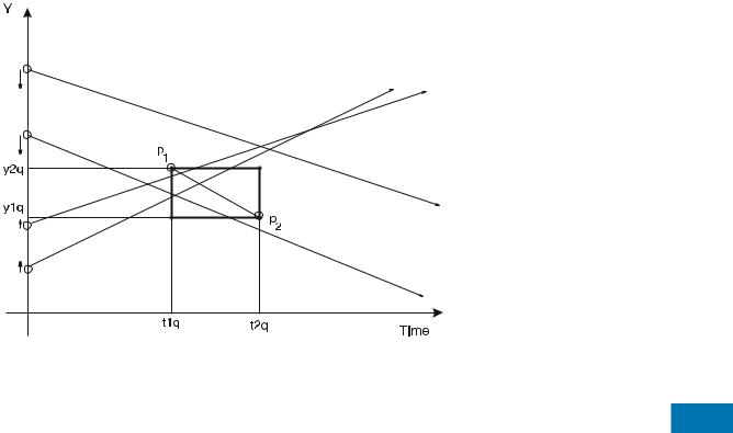
Let P(t0) = [x0, y0] be the initial position of an object at time t0. Then, the object starts moving and at time t > t0 its position will be P(t) = [x(t), y(t)] = [x0 + vx(t − t0), y0 + vy(t − t0)], where V = [vx, vy] is its velocity vector. An example for the one-dimensional case is shown in Fig. 1.
Range predictive queries in this setting have the following form: ÒReport the objects located inside the rectangle [x1q, x2q] × [y1q, y2q] at the time instants between t1q and t2q (where tnow ≤ t1q ≤ t2q), given the current motion information of all objectsÓ (i. e., the two-dimensional Moving Objects Range (MOR) query [8]).
Historical Background
The straightforward approach of representing an object moving on an one-dimensional line is by plotting the trajectories as lines in the time-location (t,y) plane (same for (t, x) plane). The equation describing each line is y(t) = vt + a, where v is the slope (velocity in this case) and a is the intercept, which is computed using the motion information (Fig. 1). In this setting, the query is expressed as the two-dimensional interval [(y1q, y2q), (t1q, t2q)] and it reports the objects that correspond to the lines intersecting the query rectangle. The space-time approach provides an intuitive representation. Nevertheless, it is problematic since the trajectories correspond to very long lines (going to inÞnity). Using traditional indexing techniques in this setting tends to reveal many drawbacks. A method that is based on this approach partitions the space into disjoint cells and stores those lines that intersect it in each cell [4,15]. The shortcoming of these methods is that they introduce replication since each line is copied into the cells that intersect it. Given that lines are typically long, the situation becomes even worse. Moreover, using space partitioning would also result in high update overhead since when an object changes its motion information, it has to be removed from all cells that store its trajectory.
Mobile Object Indexing |
663 |
Mobile Object Indexing, Figure 1
Trajectories and query in (t , y ) plane
Saltenis et al. [13] presented another technique to index moving objects. They proposed the time-parametrized R- tree (TPR-tree), which extends the R*-tree. The coordinates of the bounding rectangles in the TPR-tree are functions of time and, intuitively, are capable of following the objects as they move. The position of a moving object is represented by its location at a particular time instant (reference position) and its velocity vector. The bounding intervals employed by the TPR-tree are not always minimum since the storage cost would be excessive. Even though it would be the ideal case (if the bounding intervals were kept always minimum), doing so could deteriorate to enumerating all the enclosed moving points or rectangles. Instead, the TPR-tree uses ÒconservativeÓ bounding rectangles, which are minimum at some time point, but not at later times. The bounding rectangles may be calculated at load-time (i. e., when the objects are Þrst inserted into the index) or when an update is issued. The TPRtree assumes a predeÞned time horizon H, from which all the time instances speciÞed in the queries are drawn. This implies that the user has good knowledge of (or can efÞciently estimate) H. The horizon is deÞned as H = UI + W, where UI is the average time interval between two updates and W is the querying window. The insertion algorithm of the R*-tree, which the TPR-tree extends to moving points, aims at minimizing objective functions such as the areas of the bounding rectangles, their margins (perimeters), and the overlap among the bounding rectangles. In the case of the TPR-tree, these functions are time dependent and their evolution in [tl, tl + H] is considered where tl is the time instance when the index is created. Thus, given an objective function A(t), instead of minimizing the objec-
tive function, the integral |
tl+H A(t) dt is minimized. An |
|
|
tl |
|
improved version of the TPR-tree, called TPR*-tree, was |
|
|
proposed by Tao et al. [14]. The authors provide a prob- |
M |
|
abilistic model to estimate the number of disk accesses |
||
for answering predictive window range queries on moving objects and using this model they provide a hypothetical ÒoptimalÓ structure for answering these queries. Then, they show that the TPR-tree insertion algorithm leads to structures that are much worse than the optimal one. Based on that, they propose a new insertion algorithm, which, unlike the TPR-tree, considers multiple paths and levels of the index in order to insert a new object. Thus, the TPR*-tree is closer to the optimal structure than the TPRtree. The authors suggest that although the proposed insertion algorithm is more complex than the TPR-tree insertion algorithm, it creates better trees (MBRs with tighter parametrized extends), which leads to better update performance. In addition, the TPR*-tree employs improved deletion and node splitting algorithms that further improve the performance of the TPR-tree. The STAR-tree, introduced by Procopiuc et al. [12], is also a time-parametrized structure. It is based upon R-trees, but it does not use the notion of the horizon. Instead, it employs kinetic events to update the index when the bounding boxes start overlapping a lot. If the bounding boxes of the children of a node v overlap considerably, it re-organizes the grand children of v among the children of v. Using geometric approximation techniques developed in [1], it maintains a timeparametrized rectangle Av(t), which is a close approximation of Rv(t), the actual minimum bounding rectangle of node v at any time instant t in to the future. It provides a trade-off between the quality of Av(t) and the com-

664 Mobile Object Indexing
plexity of the shape of Av(t). For linear motion, the trajectories of the vertices of Av(t) can be represented as polygonal chains. In order to guarantee that Av(t) is an ε-
approximation of Rv(t), trajectories of the corners of Av(t)
√
need O(1/ ε) vertices. An ε-approximation means that the projection of the Av(t) on (x, t) or (y, t) planes contains the corresponding projections of Rv(t), but it is not larger than 1 + ε than the extend on the Rv(t) at any time instant. Finally, another approach to index moving objects is based on the dual transformation that is discussed in detail in the following text. In particular, the Hough-X representation of a 2D moving point o is a four-dimensional vector (x, y, vx, vy) where x and y is the location of the moving object
at the reference time tref and vx and vy is the velocity of the object projected on the x and y axes. Based on this
approach, Agarwal et al. [2] proposed the use of multilevel partition trees1 to index moving objects using the duality transform in order to answer range queries at a speciÞc time instant (i. e., snapshot queries, where t1q = t2q). They decompose the motion of the objects on the plane by taking the projections on the (t, x) and (t, y) planes. They construct a primary partition tree Tx to keep the dual points corresponding to the motion projected on the (t, x) plane. Then, at every node v of Tx, they attach a secondary partition Tyv for the points Syv with respect to the (t, y) projection, where Sv is the set of points stored in the primary subtree rooted at v. The total space used by the index is O(n logB n), where N is the number of objects, B is the page capacity and n = N / B. The query is answered by decomposing it into two sub-queries, one on each of the two projections, and taking the dual of them, σ x and σ y, respectively. The search begins by searching the primary partition Tx for the dual points, with respect to the (t, x) projection, that satisfy the query σ x. If it Þnds a triangle associated with a node v of the partition tree Tx that lies completely inside σ x, then it continues searching in the secondary tree Tyv and reports all dual points, with respect to (t, y) projection, that satisfy the query σ y. The query is satisÞed if and only if the query in both projections is satisÞed. This is true for snapshot range queries. In [2], it is shown that the query takes O(n 12 +ε + K/B) I/Os (here K is the size of the query result) and that the size of the index can be reduced to O(n) without affecting the asymptotic query time. Furthermore, by using multiple multilevel partition trees, is is also shown that the same bounds hold for the window range query. Elbassioni et al. [5] proposed a technique (MB-index) that partitions the objects along each dimension in the dual space and
1Partition trees group a set of points into disjoint subsets denoted by triangles. A point may lie into many triangles, but it belongs to only one subset.
uses B+-trees in order to index each partition. Assuming a set of N objects moving in d-dimensional space with uniformly distributed and independent velocities and initial positions, they proposed a scheme for selecting the bound-
aries of the partitions and answering the query, yielding a O(n1−1/3d (σ logB n)1/3d + k) average query time using
O(n) space ( n |
= N/B, k = |
K/B). The total number of B- |
|||
|
|
d |
|||
trees used is σ 3d s2d − 1, where σ = |
i |
1 ln(vi,max/vi,min) |
|||
|
1/d |
, where vi,max |
= |
||
and s = (n/ logB n) |
and vi,min are the |
||||
maximum and minimum velocities in dimension i respectively. The dual transformation has been adapted in [11], where the advantages over the TPR-trees methods have also been observed. Using the idea in [8], trajectories of d- dimensional moving objects are mapped into points in the dual 2d-dimensional space and a PR-quadtree is built to store the 2d-dimensional points. Similarly with [8], a different index is used for each of two reference times that change at periodic time intervals. At the end of each peri-
od, the old index is removed and a new index with a new reference point is built. Yiu et al. [17] proposed the Bdual-
tree that uses the dual transformation and maps the dual points to their Hilbert value, thereafter using a B+-tree to index the objects. That was an improvement of the method proposed by Jensen et al. [7], which indexes the Hilbert value of the locations of the moving objects (without taking into account their velocities).
Scientific Fundamentals
The Dual Space-Time Representation
In general, the dual transformation is a method that maps a hyper-plane h from Rd to a point in Rd and vice-versa. In this section, it is brießy described how the problem at hand can be addressed in a more intuitive way by using the dual transform for the one-dimensional case.
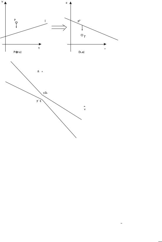
SpeciÞcally, a line from the primal plane (t, y) is mapped to a point in the dual plane. A class of transforms with similar properties may be used for the mapping. The problem setting parameters determine which one is more useful.
One dual transformation for mapping the line with equation y(t) = vt + a to a point in R2 is to consider the dual plane where one axis represents the slope of an objectÕs trajectory (i. e., velocity) and the other axis its intercept (Fig. 2). Thus, the dual point is (v, a) (this is called Hough- X transform). Similarly, a point p = (t, y) in the primal space is mapped to line a(v) = −t v + y in the dual space. An important property of the duality transform is that it preserves the above-below relationship. As it is shown in Fig. 2, the dual line of point p is above the dual point l* of the line l. Based on the above property, it is easy to show that the 1-d query [(y1q,y2q),(t1q,t2q)] becomes a polygon in the dual space. Consider a point moving with positive
Mobile Object Indexing |
665 |
Mobile Object Indexing, Figure 2 Hough-X dual transformation: primal plane (left ), dual plane (right )
|
|
n = 1v (Hough-Y). Coordinate b is the point where the line |
|
|
|
intersects the line y = 0 in the primal space. By using this |
|
|
|
transform, horizontal lines cannot be represented. Similar- |
|
|
|
ly, the Hough-X transform cannot represent vertical lines. |
|
|
|
Therefore, for static objects, only the Hough-X transform |
|
|
|
can be used. |
|
|
|
Indexing in One Dimension |
|
|
|
In this section, techniques for the one-dimensional case |
|
|
|
|
|
|
|
M |
|
|
|
are presented, i. e., for objects moving on a line segment. |
|
|
|
There are various reasons for examining the one-dimen- |
|
|
|
|
|
|
|
sional case. First, the problem is simpler and can give |
|
|
|
good intuition about the various solutions. It is also eas- |
|
|
|
ier to prove lower bounds and approach optimal solutions |
|
|
|
for this case. Moreover, it can have practical uses as well. |
|
|
|
A large highway system can be approximated as a collec- |
|
|
|
|
|
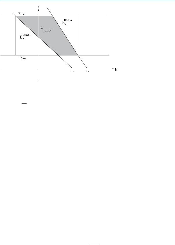
Mobile Object Indexing, Figure 3 Query on the Hough-X dual plane |
tion of smaller line segments (this is the 1.5 dimension- |
|
|
al problem discussed in [8]), on each of which the one- |
|
||
|
|
|
|
|
|
dimensional methods can be applied. |
|
velocity. Then, the trajectory of this point intersects the query if and only if it intersects the segment deÞned by the points p1 = (t1q, y2q) and p2 = (t2q, y1q) (Fig. 1). Thus, the dual point of the trajectory must be above the dual line p*2 and below p*1. The same idea is used for the negative velocities.
Therefore, using a linear constraint query [6], the query Q in the dual Hough-X plane (Fig. 3) is expressed in the following way:
If v > 0, then Q = C1 C2,
where: C1 = a + t2qv ≥ y1q and C2 = a + t1qv < qy2q
If v < 0, then Q = D1 D2,
where: D1 = a + t1qv ≥ y1q and D2 = a + t2qv < qy2q
By rewriting the equation y = vt + a as t = 1v y − av , a different dual representation can be used. Now the point in the dual plane has coordinates (b, n), where b = − av and
An (Almost) Optimal and Not Practical Solution
Matousek [9] gave an almost optimal algorithm for simplex range searching given a static set of points. This main memory algorithm is based on the idea of simplicial partitions.
For a set S of N points, a simplicial partition of S is a set {(S1, 1), . . . (Sr , r)} where {S1, . . . , Sr } is a partitioning of S and i is a triangle that contains all the points in Si. If maxi|Si| < 2 mini|Si|, where |Si| is the cardinality of the set Si, the partition is balanced. Matousek [9] shows that, given a set S of N points and a parameter s (where 0 < s < N/2), it can be constructed in linear time a balanced
simplicial partition for S of size O(s) such that any line
√
crosses at most O( s) triangles in the partition.
This construction can be used recursively to construct a partition tree for S. The root of the tree contains the whole set S and a triangle that contains all the points. Then, a balanced simplicial partition of S of size √|S| is found.
666 Mobile Object Indexing
Mobile Object Indexing, Figure 4 Query on the dual Hough-Y plane
Each of the children of the root are associated with a set Si from the simplicial partition and the triangle i that contains the points in Si. For each of the SiÕs, simplicial partitions of size √|Si| are computed and continue to until each leaf contains a constant number of points. The construction time is O(N log2 N).
To answer a simplex range query, the procedure starts at the root. Each of the triangles in the simplicial partition at the root checks if (i) it is inside the query region, (ii) it is outside the query region or, (iii) it intersects one of the lines that deÞne the query. In the Þrst case, all points inside the triangle are reported and in the second case the triangle is discarded, while in the third case it continues the recursion on this triangle. The number of triangles that the query can cross is bounded since each line crosses at most O(|S|1/4) triangles at the root. The query time is O(N1/2+ε ), with the constant factor depending on the choice of ε.
Agarwal et al. [2] gave an external memory version of static partition trees that answers queries in O(n1/2+ε + k) I/Os. The structure can become dynamic using a standard technique by Overmars [10].It can be shown that a point is inserted or deleted in a partition tree in O(log22 N) I/Os and answer simplex queries in O(n1/2+ε + k) I/OÕs. A method that achieves O(log2B( NB )) amortized update overhead is presented in [2].
Using Point Access Methods Partition trees are not very useful in practice because the query time is O(n1/2+ε + k) and the hidden constant factor becomes large for small ε. In this section, two different and more practical methods are presented.
There are a large number of access methods that have been proposed to index point data. All of these structures were designed to address orthogonal queries, i. e., a query
expressed as a multidimensional hyper-rectangle. However, most can be easily modiÞed to address non-orthogonal queries like simplex queries.
Goldstein et al. [6] presented an algorithm to answer simplex range queries using R-trees. The idea is to change the search procedure of the tree. In particular, they gave efÞcient methods to test whether a linear constraint query region and a hyper-rectangle overlap. As mentioned in [6], this method is not only applicable to the R-tree family, but to other access methods as well. This approach can be used to answer the one-dimensional MOR query in the dual Hough-X space.
This approach can be improved by using a characteristic of the Hough-Y dual transformation. In this case, objects have a minimum and maximum speed, vmin and vmax, respectively. The vmax constraint is natural in moving object databases that track physical objects. On the other hand, the vmin constraint comes from the fact that the Hough-Y transformation cannot represent static objects. For these objects, the Hough-X transformation is used, as it is explained above. In general, the b coordinate can be computed at different horizontal (y = yr) lines. The query region is described by the intersection of two half-plane
|
|
|
|
|
|
|
|
|
|
|
|
|
|
|
|
|
|
1 |
|
||
queries (Fig. 4). The Þrst line intersects the line n = |
|
|
|
||||||||||||||||||
vmax |
|||||||||||||||||||||
|
|
|
|
|
|
y2q−yr |
|
|
1 |
|
|
|
|
|
|
|
1 |
|
|||
at the point (t1q − |
|
vmax |
|
, |
vmax |
) and the line n |
= |
vmin |
|
||||||||||||
at the point (t1q − |
y2q−yr |
, |
|
|
1 |
). Similarly, the other line |
|||||||||||||||
|
vmin |
|
vmin |
||||||||||||||||||
that deÞnes |
the query intersects the |
horizontal |
lines at |
||||||||||||||||||
(t2q − |
y1q−yr |
, |
1 |
) and (t2q |
− |
|
y1q−yr |
, |
1 |
). |
|
|
|
|
|||||||
vmax |
vmax |
|
|
vmin |
|
vmin |
rectan- |
||||||||||||||
Since |
access |
methods are |
more |
efÞcient for |
|||||||||||||||||
gle queries, suppose that the simplex query is approximated with a rectangular one. In Fig. 4, the query
approximation |
rectangle will be [(t1q − |
y2q−yr |
, t2q |
− |
|||||
vmin |
|||||||||
|
y1q−yr |
), ( |
1 |
, |
1 |
)]. Note that the query area is enlarged |
|||
|
|
|
|
||||||
|
vmax |
vmax |
vmin |
|
|
|
|||
Mobile Object Indexing |
667 |
|
|
|
|
|
|
|
|
|
|
|
|
|
|
|
|
|
|
|
|
|
|
|
|
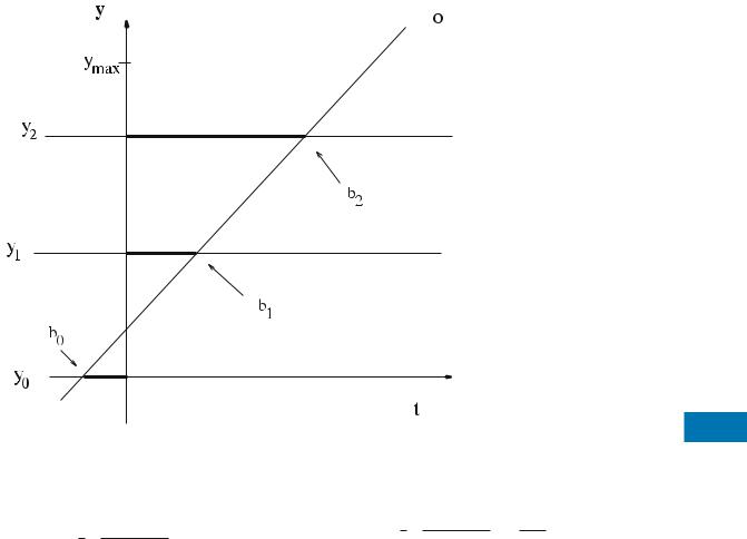
Mobile Object Indexing, Figure 5 |
|
||
|
|
|
|
|
|
|
|
|
|
|
|
|
|
|
|
|
|
|
|
|
|
|
|
Coordinate b as seen from different Ôobser- |
|
||
|
|
|
|
|
|
|
|
|
|
|
|
|
|
|
|
|
|
|
|
|
|
|
|
vationÕ points |
M |
||
|
|
|
|
|
|
|
|
|
|
|
|
|
|
|
|
|
|
|
|
|
|
|
|
|
|
|
|
by the area E = E |
HoughY |
= E1 |
HoughY |
+ E2 |
HoughY |
, which is |
(i) y2q − y1q |
< q |
ymax |
|
|
|
|||||||||||||||
|
|
|
|
|
|
|
|
c : then it can be easily shown that |
|||||||||||||||||||
computed as: |
|
|
|
|
|
|
|
|
|
|
|
|
|
|
|
|
|
|
area E is bounded by: |
|
|
|
|||||
|
|
|
vmax − vmin |
2 |
|
|
|
|
|
|
|
|
|
|
|
|
|
|
E < q 1 |
vmax − vmin |
2 |
ymax . |
|
||||
EHoughY |
= |
1 |
( |
| |
y |
2q − |
y |
r | + | |
y |
1q − |
y |
r | |
) |
|
(2) |
||||||||||||
|
2 |
|
vmin · vmax |
|
|
|
|
|
|
|
|
2 |
|
vmin · vmax |
|
c |
|
||||||||||
(1)The query is processed at the index that minimizes |y2q −
The objective is to minimize E since it represents a mea- |
yr| + |y1q − yr|. |
ymax |
||
(ii) y2q − y1q > |
c : the query interval contains one or |
|||
sure of the extra I/OÕs that an access method will have to |
more sub-terrains, which implies that if a query is execut- |
|||
perform for solving a one-dimensional MOR query. E is |
ed at a single observation index, area E becomes large. To |
|||
based on both yr (i. e., where the b coordinate is comput- |
bound E, index each sub-terrain too. Each of the c sub- |
|||
ed) and the query interval (y1q, y2q), which is unknown. |
terrain indices records the time interval when a moving |
|||
Hence, the method keeps c indices (where c is a small con- |
object was in the sub-terrain. Then, the query is decom- |
|||
stant) at equidistant yrÕs. All c indices contain the same |
posed into a collection of smaller sub-queries: one sub- |
|||
information about the objects, but use different yrÕs. The |
query per sub-terrain fully contained by the original query |
|||
i-th index stores the b coordinates of the data points using |
interval, and one sub-query for each of the original queryÕs |
|||
yi = |
ymax |
· i, i = 0, . . . , c − 1 (see Fig. 5). Conceptually, |
endpoints. The sub-queries at the endpoints fall to the case |
|
c |
||||
yi serves as an ÒobservationÓ element and its correspond- |
(i) above, thus, they can be answered with bounded E using |
|||
ing index stores the data as observed from position yi. The |
an appropriate ÒobservationÓ index. To index the intervals |
|||
area between subsequent ÒobservationÓ elements is called |
in each sub-terrain, an external memory interval tree can |
|||
a sub-terrain. A given one-dimensional MOR query will |
be used which answers a sub-terrain query optimally (i. e., |
|||
be forwarded to, and answered exactly by, the index that |
E = 0). As a result, the original query can be answered with |
|||
minimizes E. |
bounded E. However, interval trees will increase the space |
|||
To process a general query interval [y1q, y2q], two cases |
consumption of the indexing method. |
|||
are considered, depending on whether the query interval |
The same approach can be used for the Hough-X transfor- |
|||
covers a sub-terrain: |
mation, where, instead of different ÒobservationÓ points, |
|||
668 Mobile Object Indexing
Mobile Object Indexing, Figure 6
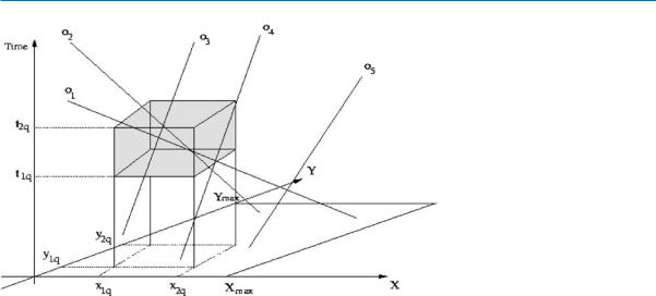
Trajectories and query in (x ,y ,t ) space
different ÒobservationÓ times are used. That is, the intercept a can be computed using different vertical lines t = ti, i = 0, . . . , c − 1. For each different intercept, an index is created. Then, given a query, one of the indices is chosen to answer the query (the one that is constructed for the ÒobservationÓ time closest to the query time.) However, note that if the query time(s) is far from the ÒobservationÓ time of an index, then the index will not be very efÞcient since the query in the Hough-X will not be aligned with the rectangles representing the index and the data pages of this index. Therefore, one problem with this approach comes from the fact that the time in general and the query time in particular, are always increasing. Therefore, an index that is efÞcient now will become inefÞcient later. One simple solution to this problem is to create a new index with a newer observation time every T time instants, at the same time removing the index with the oldest observation time [8,11]. Note that this problem does not exist in the Hough-Y case since the terrain and the query domain do not change with time (or they change very slowly).
Indexing in Two Dimensions
For the two-dimensional problem, trajectories of the moving objects are lines in a three dimensional space (see Fig. 6). Thus, the dual transformation gives a 4-dimension- al dual point. Another approach is to split the motion of an object into two independent motions, one in the (t, x) plane and one in the (t, y) plane. Each motion is indexed separately. Next, the procedure used to build the index is presented as well as the algorithm for answering the 2-d query.
Building the Index The motion in (x, y, t) space is decomposed into two motions, one on the (t, x) and the other on the (t, y) plane. Furthermore, on each projec-
tion, the objects are partitioned according to their velocity. Objects with small velocity magnitudes are stored using the Hough-X dual transform, while the rest are stored using the Hough-Y transform, i.e, into distinct index structures.
The reason for using different transforms is that motions with small velocities in the Hough-Y approach are mapped into dual points (b, n), having large n coordinates (n = 1v ). Thus, since few objects have small velocities, by storing the Hough-Y dual points in an index structure such an R*-tree, MBRs with large extents are introduced and the index performance is severely affected. On the other hand, by using a Hough-X index for the small velocitiesÕ partition, this effect is eliminated since the Hough-X dual transform maps an objectÕs motion to the (v, a) dual point. The objects are partitioned into slow and fast using a threshold VT.
When a dual point is stored in the index responsible for the objectÕs motion in one of the planes, i. e., (t, x) or (t,y), information about the motion in the other plane is also included. Thus, the leaves in both indices for the Hough-Y partition store the record (nx, bx, ny, by). Similarly, for the Hough-X partition in both projections, the record (vx, ax, vy, ay) is stored. In this way, the query can be answered by one of the indices; either the one responsible for the (t, x) or the (t, y) projection.
On a given projection, the dual points (i. e., (n, b) and (v, a)) are indexed using R*-trees [3]. The R*-tree has been modiÞed in order to store points at the leaf level and not degenerated rectangles. Therefore, extra information about the other projection can be stored. An outline of the procedure for building the index follows:
1.Decompose the 2-d motion into two 1-d motions on the (t, x) and (t, y) planes.
Mobile Object Indexing |
669 |
2.For each projection, build the corresponding index QHoughY. Similarly, on the dual Hough-X plane (Fig. 3),
structure.
2.1Partition the objects according to their velocity:
Objects with |v| < VT are stored using the Hough-X dual transform, while objects with |v| ≥ VT are stored
using the Hough-Y dual transform.
2.2Motion information about the other projection is also included in each point.
In order to choose one of the two projections and answer the simplex query, the following technique is used.
Answering the Query The two-dimensional MOR query is mapped to a simplex query in the dual space. The simplex query is the intersection of four 3-d hyperplanes and the projections of the query on the (t, x) and (t, y) planes are wedges, as in the one-dimensional case.
The 2-d query is decomposed into two 1-d queries, one for each projection, and it is answered exactly. Furthermore, on a given projection, the simplex query is processed in both partitions, i. e., Hough-Y and Hough-X.
On the Hough-Y plane the query region is given by the intersection of two half-plane queries, as shown in Fig. 4. Consider the parallel lines n = and n = . Note that a minimum value for vmin is VT. As illustrated in Sect. 2, if the simplex query was answered approximately, the query area would be enlarged by
(the triangular areas in actual area of the simplex query be
let QHoughX be the actual area of the query and EHoughX be the enlargement. The algorithm chooses the projection which minimizes the following criterion κ:
κ = |
EHoughY |
+ |
EHoughX |
(3) |
|
|
|
. |
|||
QHoughY |
QHoughX |
||||
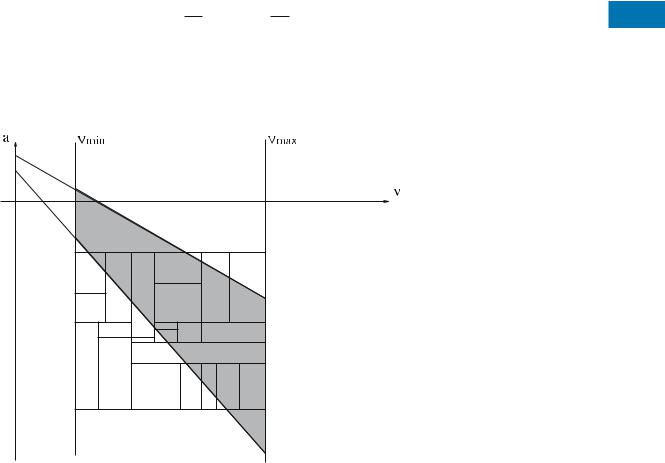
The intuition for this heuristic is that simplex queries in the dual space are not aligned with the MBRs of the underlying index (see Fig. 7). Therefore, the projection where the query is as much aligned with the MBRs as possible is chosen. The empty space, as used in the aforementioned criterion deÞnition, gives an indication of that.
Since the whole motion information is kept in the indices, it can be used to Þlter out objects that do not satisfy the query. An outline of the algorithm for answering the exact 2-d query is presented below:
1.Decompose the query into two 1-d queries, for the (t, x) and (t, y) projection.
2.Get the dual query for each projection (i. e., the simplex query).
3.Calculate the criterion κ for each projection and choose
the one (say p) that minimizes it. |
M |
4.Answer the query by searching the Hough-X and Hough-Y partition using projection p.
5.Put an object in the result set only if it satisÞes the query. Use the whole motion information to do the Þltering Òon the ßyÓ.
Mobile Object Indexing, Figure 7 Simplex query in dual space, not aligned with MBRs of underlying index

670 Mobile Objects Databases
Key Applications
Location-aware applications such as trafÞc monitoring, intelligent navigation, and mobile communications management require the storage and retrieval of the locations of continuously moving objects. For example, in a company that manages taxi services, a customer may want to Þnd the taxis that will be in a speciÞc area in the near future. This can be achieved by issuing a query: ÒReport the taxis that will be in the area around the customer in the next 5 minutesÓ. Similarly, in an air-trafÞc control system, the locations of the airplanes that are ßying close to an airport or a city must be continuously monitored. In that case, a predictive range query can be periodically issued every few seconds. The index will speed up the search and allow for multiple queries to be executed each minute.
Future Directions
There are a number of interesting future problems related to the discussed topic. The dual transformation has been used for objects moving in one and two dimensions. It is interesting to investigate how these methods will be extended to three or higher dimensions. Although the described methods can be applied on higher dimensions, it is not clear if they will have the same efÞciency and practicality. Most of the work has been done for linearly moving objects. An interesting future direction is to consider storage and retrieval of non-linear movements. Another problem is to consider moving objects with extents that change over time in addition to their location.
Recommended Reading
1.Agarwal, P., Har-Peled, S.: Maintaining Approximate Exten Measures of Moving Points. In: Proceedings of the 12th ACMSIAM Sympos. Discrete Algorithms, Washington, DC, USA, 7Ð9 Jan 2001, pp. 148Ð157
2.Agarwal, P.K., Arge, L., Erickson, J.: Indexing Moving Points. In: Proceedings of the 19th ACM Symp. on Principles of Database Systems, Dallas, Texas, USA, 15Ð17 May 2000, pp. 175Ð186
3.Beckmann, N., Kriegel, H., Schneider, R., Seeger, B.: The R*- tree: An EfÞcient and Robust Access Method for Points and Rectangles. In: Proceedings of the 1990 ACM SIGMOD, Atlantic City, May 1998, pp. 322Ð331
4.Chon, H.D., Agrawal, D., Abbadi, A.E.: Query Processing for Moving Objects with Space-Time Grid Storage Model. In: Proceedings of the 3rd Int. Conf. on Mobile Data Management, Singapore, 8Ð11 Jan 2002, pp. 121Ð126
5.Elbassioni, K., Elmasry, A., Kamel, I.: An efÞcient indexing scheme for multi-dimensional moving objects. In: Proceedings of the 9th Intern. Conf. ICDT, Siena, Italy, 8Ð10 2003, pp. 425Ð439
6.Goldstein, J., Ramakrishnan, R., Shaft, U., Yu, J.: Processing Queries By Linear Constraints. In: Proceedings of the 16th ACM PODS Symposium on Principles of Database Systems, Tucson, Arizona, USA, 13Ð15 May 1997, pp. 257Ð267
7.Jensen, C.S., Lin, D., Ooi, B.C.: Query and Update EfÞcient B+- Tree Based Indexing of Moving Objects. In: VLDB, Toronto, Canada, 29 Aug Ð 3 Sept 2004, pp. 768Ð779
8.Kollios, G., Gunopulos, D., Tsotras, V.: On Indexing Mobile Objects. In: Proceedings of the 18th ACM Symp. on Principles of Database Systems, Philadelphia, Pennsylvania, USA, 1Ð3 June 1999, pp. 261Ð272
9.Matousek, J.: EfÞcient Partition Trees. Discret. Comput. Geom. 8, 432Ð448 (1992)
10.Overmars, M.H.: The Design of Dynamic Data Strucutures. vol. 156 of LNCS. Springer-Verlag, Heidelberg (1983)
11.Patel, J., Chen, Y., Chakka, V.: STRIPES: An EfÞcient Index for Predicted Trajectories. In: Proceedings of the 2004 ACM SIGMOD, Paris, France, 13Ð18 June 2004, pp. 637Ð646
12.Procopiuc, C.M., Agarwal, P.K., Har-Peled, S.: Star-tree: An efÞcient self-adjusting index for moving objects. In: Proceedings of the 4th Workshop on Algorithm Engineering and Experiments, San Francisco, CA, USA, 4Ð5 Jan 2002, pp. 178Ð193
13.Saltenis, S., Jensen, C., Leutenegger, S., Lopez, M.A.: Indexing the Positions of Continuously Moving Objects. In: Proceedings of the 2000 ACM SIGMOD, Dallas, Texas, USA, 16Ð18 May 2000, pp. 331Ð342
14.Tao, Y., Papadias, D., Sun, J.: The TPR*-Tree: An Optimized Spatio-temporal Access Method for Predictive Queries. In: Proceedings of the 29th Intern. Coonf. on Very Large Data Bases, Berlin, Germany, 9Ð12 Sept 2003, pp. 790Ð801
15.Tayeb, J., Olusoy, O., Wolfson, O.: A Quadtree-Based Dynamic Attribute Indexing Method. Comp. J., 41(3), 185Ð200 (1998)
16.Wolfson, O., Xu, B., Chamberlain, S., Jiang, L.: Moving Objects Databases: Issues and Solutions. In: Proceedings of the 10th Int. Conf. on ScientÞc and Statistical Database Management, Capri, Italy, 1Ð3 July 1998, pp. 111Ð122
17.Yiu, M.L., Tao, Y., Mamoulis, N.: The Bdual-Tree: Indexing Moving Objects by Space-Filling Curves in the Dual Space. VLDB J., To Appear
Mobile Objects Databases
HARVEY J. MILLER
Department of Geography, University of Utah, Salt Lake City, UT, USA
Synonyms
Moving objects database
Definition
Mobile objects databases (MOD) store data about entities that can change their geometry frequently, include changes in location, sizes and shapes
Main Text
Most database management systems (DBMS), even spatiotemporal DBMS, are not well equipped to handle data on objects that change their geometry frequently, in some cases continuously. In DBMS, data is assumed to be constant