7.2.3. Computer experiment

Model we built is implemented in Objective - C multi-agent simulation system SWARM. Capabilities built graphical user interface in this package allow you to visually observe the development process. With the help of special tools contained in the main library , we display an animated picture. Research findings to (grid area) on which are located the family, consisting of agent - men and women - agent, and displays the number of the resource in each cell. Cells containing the family of agents with different identities , have different colors . Degree of resource wealth in the sources of the medium varies in color : the more resource , the brighter the color. Thus, we can identify a rich source of income. Process can be observed in both continuous and single-stepping. At any time, you can learn the value of family characteristics, the identity of agents causing accessory graphics window for each family. By changing the value in the window parameters, we are able to move the family to another source of income, to change its characteristics.

Upon initial startup of a program model appears custom control panel that can switch modes (stop, continuous and single-step mode , preserving any stage of simulation ) , the initial panel data model , displaying the initial values ​​of the parameters that are set by the researcher.

For the model described above carried out computer experiments chosen values ​​of the characteristics for which the agents' behavior is consistent with a simulated situation. There was Discussed the behavior of the family before, during and after the economic crisis. Initially, the model is given the pre-crisis situation, with family- oriented way of life of family members, the expected adoption by both men and women's traditional roles , i.e. man works and the woman asked .

Figure 7.1. Stage of family life in a stable society.

Families are distributed randomly , having certain intrinsic characteristics : initial capital , the level of adaptation , tolerance, the degree of identity of women in the family , the coefficients of income men, women and family consumption . Examined 50 families (Figure 7.1) . The dots appear families with two working spouses, light - families in which the husband provides the family completely. Around agents with different brightness squares characterize resource availability in the sources of household income. At intervals that decrease resource occurs in the sources of household income, the increase . The task of the agents is to maintain a balance between income and consumption of resources in the family.

During most of the revenue growth agents female oriented family (Figure 7.1). But there comes a time when a sharp decline in resources in sources of income leads to the economic crisis in the family. In this case, agents need to navigate and select the most appropriate strategy for their seven adaptive behavior . It may be:

1. The search for more money work (agents move closer to the locations of the richest resources);

2. Reduction claims (agents forced due to an acute shortage of income to reduce their costs);

3. Change of identity - female agent with high personal activity can change in the time of crisis the family orientation to professional.

Figure 7.2. Families’ artificial society in a state of economic crisis.

You can see that in the case of a long economic crisis, most agents are women professional orientation ( Figure 7.2 ) . If the strategy of adaptive economic behavior is selected successfully, these families set the balance of growth and resource consumption .

After some time, you can observe the change of the initial capital, the flow coefficient of the family, self-identity of women , the number of families overcome a crisis situation , as well as an increase / decrease in the share of income sources with a certain period . We can set time periods of economic crisis and sustainable development. In this example, the period is 400 . So first we set stage of stable development of society, and then in a period of economic crisis, etc.

Figure 7.3. Dynamics of changes in equity of the family.

Figure.7.4. graph of change the flow coefficient of family capital.

Figure 7.3. Given the dynamics of family capital . The time interval (0.400) observed vibration capital growth family. At the time (given the time of onset of the economic crisis) is a sharp decrease in available capital. Life is getting more expensive, and less income ( the amount of resource with the onset of the crisis in the sources of income decreases). At the end of the economic crisis gradually begins to increase capital of the family.

On figure 7.4. Graph changes the flow coefficient of family capital in time . During the period of stable development (0.400) flow coefficient increases family in accordance with the cash capital increase family (Figure 7.3) and eventually stabilizes. With the onset of the economic crisis (small number of families reduce their costs, but most adhere to the old flow coefficient, i.e. they try to keep the old way of life. But at the time () when the capital of the family (Figure 7.3) falls below a given limit, signifying a severe economic crisis in the family , the main number of families forced to drastically reduce their costs. After the economic crisis while the flow coefficient is stored small family. This is because families are still waiting for what life will be difficult financially, and fear whether they can adapt if, immediately increase their costs.

Later, when the capital of the family income exceeds the average border , the family gradually begins to increase spending . But not to the level seen before the economic crisis. Therefore, initially, during the crisis, most families do not want to part with a primary standard of living and using internal resources of the family, opting for strategies of adaptive behavior, as the search for more money and work expectant strategy. We can conclude that strategy. We can conclude that a strategy to reduce costs required family in a situation of acute economic crisis.

Fig. 7.5. Graph of the number of families.

On Fig.7.5. given a graph of the number of households over time. The graph shows that the number of families in crisis for some time maintained (there is a choice of different strategies of adaptive behavior), but later, when the capital of the family is much below the subsistence level and not successful survival strategy, the family is on the "edge" of sustainability, and degrades a number of families. With the cessation of the economic crisis the number of families again stabilized.

Fig.7.6. chart the ratio of families with different identities of women.

On fig.7.6 chart reflects the change in the ratio of families with professional and family identity of women. First column shows the number of families in which family-oriented woman, the second - a professionally-oriented. Analyze when change occurs in women in the family identity. From the diagram on fig.7.6 we can see that that most women do not work before the crisis in accordance with traditional family.

Fig.7.7: correlation diagram when an economic crisis.

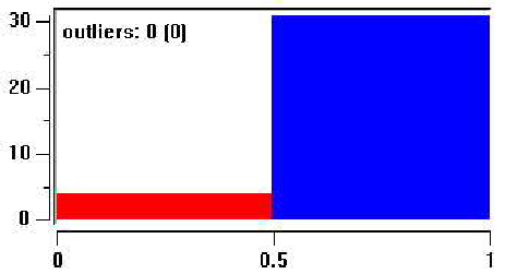
Fig .7.8: diagram relations in time of acute crisis.

fig.7.9: chart correlations in overcoming the economic crisis.

Fig.7.10: chart relations on stable development stage.

With the economic downturn, an increasing proportion of professionally-oriented women ( fig.7.7 ) . during the period of acute crisis vast majority of women are forced to work . Here the husband and wife share responsibility for financial provision for the family ( fig.7.8 ) .

The strategy of " housewife " is formed as overcoming the economic crisis and achieve stability in society (fig.7.9 ) . Later , at the stage of stable development of society , clearly outweighed the scales towards families in which women do not work because the income of her husband provides a high standard of living (fig.7.10 ) .

These results suggest not only on the proportion of a particular strategy , but about family behavior trends in an effort to overcome the crisis situation . The observed difference in the study strategies shows that the main internal reserve when an economic crisis, which tries to use the family is a woman's ability to change the orientation of the professional family . This gives an additional income for the family and an opportunity to overcome the economic crisis .

2.2 Model " predator-prey "

Consider another form of coexistence between the two species , when the first of them is the food for a second . If in a given environment inhabited only the first type ( the victim ) , it would have natural growth, which is considered constant and positive (assuming that the victim is no shortage of food .) Then in the absence of predators would be observed exponential growth in the number of victims. If the second form of predators exist in isolation , it is due to lack of food (ie victims) he would have had negative growth numbers - extinction ratio in the absence of predators victims. Outcome here would be complete extinction of predators.

The coexistence of species in a limited area , they have a strong influence on each other . Obviously , the increase in the number of victims should be reduced , and the more , the higher the number of predators. This is explained by the fact that more needs to predators appropriate amount of food which have to act as long-suffering victims. On the other hand , the increase in predators should increase the stronger , the higher the number of victims , because in these conditions a greater number of predators will be providing nutritious food . As a result, we obtain the differential equation

Where the coefficients and describes the changes in growth of praise and predators due to their natural interaction between them. Equation with appropriate initial conditions forms a well-known mathematical model of "predator-prey".

To study the resulting system will use a fairly common technique associated with a change of variables. Define the quantities

Where the constants a, b ​​and c are chosen so that the resulting equations were as simple as possible look. As a result, we establish relations

(6.8)

Where ,.

Define parameters

We obtain the relations

(6.9)

It is called Volterra-Lotka equations System (6.9) and (6.8) have the same meaning. Indeed function and status, as well as the independent variable is different from the values ​​and t, respectively, only by constant factors. Thus, we still have to deal with the number of species and the time, but dealt with in a different scale.

Obviously, equation (6.9) has two equilibrium positions . The first bottom trivially implemented in the absence of both species and is of no practical interest. Much more interesting second equilibrium of the system. Here, the number of newly born while their victims compensated number, eaten at the same time predators. In turn, predator’s fertility and mortality is also the same. Consequently, the number of both species over time does not change, i.e. the system is in a state of dynamic equilibrium.

Consider the behavior of the studied system is the equilibrium position. Note that the number of species known to be negative. The vanishing of the primary predators with a positive initial prey population leads to an equation whose solution will increase exponentially. Thus, in the absence of natural enemies and victims of food restriction on indefinitely multiply. Lack of victims at the initial time allow to obtain the following equation For the number of predators, it follows that there is no food predators gradually die. For further research is sufficient to consider positive initial states.

As can be seen from equations (6.9), there are four areas in the phase plane, which differ among themselves in terms of the behavior of the system (Fig. 38). If at some time t the inequalities

0<u(t)<1, 0<v(t)<1, (6.10)

The right side of the first equation (6.9) is positive and the second negative. Then the inequalities and thus, the function u will increase over time, and v - to decrease. (Fig. 39)

Fig. direction of evolution of the system model

Such behavior of the system is maintained as long as the relations ( 6.10). These conditions can be broken or in the case where the process of increasing the value of u exceeds unity, or when the function v zero as its decrease. However, the approach of the value of v to zero, its derivative will be in accordance with the second equation (6.9). Thus achieving zero function v could only be asymptotic. However, with increasing and decreasing functions u v derivative not only remains positive, but even increasing. Therefore, sooner or later, the value of u exceeds unity, and we find ourselves in an area characterized by the inequalities

Changing the number of prey and predators at the parameter values

Under these conditions, the derivatives of both functions are positive, and thus, their values ​​will increase with time. This behavior can occur as long as the relations (6.11). Obviously, with an increase in the functions it ever exceeds unity, and the resulting conditions are met

(6.12)

In the future, there is decrease of the function while increasing value. The situation changed only in case of violation of one of the ratio (6.12). Naturally, in descending order in the end it will be less than unity, and the inequalities

(6.13)

This means that both the functions are decreasing. Given that as the function tends to zero to zero and its derivative, we conclude that sooner or later the time when the function will be less than unity for a positive value. Thus, again the following relations (6, 10) and hence described process is performed.

We can establish that the solutions of equations (6.9) are periodic functions (Fig. 40). In the phase plane, they correspond to closed curves. With this type of equilibrium position (center) we have already met in the study of free undammed mechanical and electrical oscillations. At the same time, the trivial equilibrium position ( the origin in the phase plane ) have fundamentally different properties. Obviously, it tends to only those states that lie on the reference axis in the phase plane. Others may phase curves while approaching to the origin , but later inevitably move away from it . Thus we are dealing with an unstable equilibrium position, which is a saddle.