Linear Engine / L2V4bGlicmlzL2R0bC9kM18xL2FwYWNoZV9tZWRpYS83MTc1

components should be the dominant design parameters on the engine’s operating frequency, which is largely influenced by the weight of the translator.

8.2 The effect of stroke length

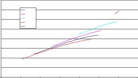
Simulation was performed to investigate the effect of stroke length on operating frequency, peak cylinder pressure, and compression ratio. Note should be taken that it was not effective stroke length that was investigated in this case. Effective stroke length was kept constant at 38 mm. A representative of total stroke length is free travel that was defined in Section 7.3. Table 10 and Figure 80 show the results of the simulation. Increasing the free travel decreased the operating frequency and the compression ratio as was expected. As the free travel increased, it took a longer time for the translator to travel from BDC to TDC. This resulted in lowered operating frequency and compression ratio. The surprising phenomenon was that decreased free travel resulted in decreased peak pressure. This needs further investigation for a feasible explanation.

Table 10. The effect of free travel on operating frequency, peak pressure, and compression ratio. Fuel injected was 40 µl/injection at 10 mm before TDC.

143

Free travel of the translator (mm)

Figure 80. The effect of free travel on operating frequency, peak pressure, and compression ratio. Fuel injected was 40 µl/injection at 10 mm before TDC.

8.3 The effect of the amount of fuel injected

The experimental data were not sufficient to examine the effect of the amount of fuel injected on engine behavior. However, the initial testing of the engine suggested that operating frequency was insensitive to the amount of fuel injected into the cylinder. This would have meant that the engine had a narrow window of preferred frequency of operation. Further investigation determined that the engine was controlled by the amount of air rather than the amount of fuel in the cylinder during those initial test runs. The uncertainty about the fuel amount-frequency relationship required the simulation study of the area. For this study the amount of fuel injected into the cylinder was gradually decreased until the engine was unable to sustain operation. Figure 81 shows the effect of

144

the amount of fuel injected on frequency. It is obvious that more fuel resulted in higher operating frequency. It was also clear, as it can also be seen in the results in Section 8.1, that an engine with greater translator mass has a better ability to sustain operation. An engine with larger translator mass is able to sustain operation on less fuel than an engine with a lighter translator. In the simulation, an engine with a 2.8 kg translator was able to operate on as low as 3.5 µl/injection, while the engine with a 4.7 kg translator was able to

operate on as little fuel as 2.3 µl/injection resulting in 49 Hz and 35 Hz respectively. These numbers were around experimental data, 50Hz and 35 Hz, which proves that the engine during the first test runs, where much more fuel was injected into the cylinder, was severely under scavenged. The required fuel to create stochiometric air-fuel ratio would be 12.2 µl/injection, assuming 100 % volumetric efficiency.

Fueling rate (microliter/injection)

Figure 81. Engine operating frequency vs. amount of fuel injected. No load was applied. Heat release was instantaneous.

145

Figure 82 shows the lowest operating frequency vs. translator mass. Fuel amount

injected was different for each data point.

Translator mass (kg)

Figure 82. Lowest operating frequency vs. translator mass. Fuel amount injected was different for each data point.

8.4 The effect of injection timing

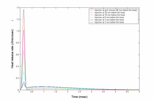
For examining the effect of injection timing, the heat release rate (Wiebe function) was varied as a function of injection timing. The heat release rates used in the simulation for different injection timings can be seen in Figure 83. It is clear that even very early injection would not result in perfect HCCI operation but the aim of this part of the study was to show the benefits of the HCCI operation therefore fuel injection at 38 mm before the head was chosen to represent pseudo-HCCI operation. In the case of early injection the burning happens completely in the premix burn regime. Van Blarigan et al. [74] reported that 95% of the fuel is burned in 80 µs. A value of 150 µs burning time

146

was chosen for the pseudo-HCCI operation to compensate for the effect of possible imperfect mixing. The late injection, 3 mm before the head, represents regular DICI operation with 10% premix burn in 150 µs and total burning time of 5 ms. Between the two extreme cases, pseudo-HCCI and DICI, the ratio of the fuel burned in premix burn and the diffusion part of the burn was varied as a linear function of injection timing.

Figure 83. Heat release rates for different injection timings were calculated by using double Wiebe functions.

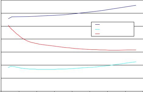
Injection timing was varied in the simulation model to determine the effect of injection timing on operating frequency, compression ratio, and peak cylinder pressure. The simulation was run with no load and 40 µl fuel/injection. The results are summarized in Table 11 and visualized in Figure 84.

147

Table 11. The effect of injection timing on operating frequency, compression ratio, and peak cylinder pressure.

Injection timing (mm before TDC)

Figure 84. Operating frequency, peak pressure, and compression ratio vs. injection timing.

Advanced injection timing resulted in increased frequency and decreased compression ratio. Peak cylinder pressure was high for late and early injection with a decreased value in between. This was believed to be due to the following: as timing was advanced until about 10 mm before TDC, the heat release rate did not change much but the cylinder temperature was elevated for a longer period of time resulting in higher heat loss and lowered pressure than those in the case of late injection. Advancing the timing further, resulted in a larger portion of the heat release in premix burn that yielded a more sudden rise in pressure that yielded increased efficiency because of the HCCI operation.

148

This phenomenon suggests that advancing injection timing marginally will not have the desired pseudo-HCCI effect on engine operation, it can even result in an efficiency drop. This suggests that fuel volatility is an important feature in terms of linear engines. It also suggests that the injector should be placed in the intake or scavenging duct to ensure thorough mixing and evaporation for HCCI operation.

8.5 Effect of load

The effect of load on operating frequency is shown in Figure 85. The amount of fuel injected was kept constant at 40 µl/injection at 10 mm before TDC. Load was gradually increased until the engine stalled. Increasing the load caused the frequency to decrease. This effect was not unexpected as increasing load and decreasing fueling reduces the speed in conventional engines as well. However, the frequency of the linear engine as the function of load and fueling rate did not change as dramatically as it would in slider crank engines. This was mainly due to the fact that lowering the load and/or increasing fueling rate resulted higher operating frequency as well as higher compression ratio. The higher compression ratio yielded higher temperature and increased heat loss to the cylinder walls. Trends were similar for both simulation and real engine operation. The fact that increasing load reduces and increasing fueling rate increases the operating frequency makes operating frequency the obvious choice for a feedback parameter to control fuel quantity injected into the cylinder.

149

Figure 85. The effect of load on operating frequency.

8.6 Results of the predictor/simulator model

The predictor/simulator was created to find the set of engine parameters that yielded the highest mechanical efficiency. The predictor/simulator used a genetic algorithm and a neural network along with the simulation model in a recursive process. Section 5.2 described the model in detail and the results are described here.

Figure 86 shows the predicted efficiency and simulated efficiency for the iterative predicting/simulating process. The first fifty points were the initial randomly selected sets of engine parameters. It can be seen from the figure that predicted efficiency was always around 45-50% while the simulated efficiency varied between 10-45 %. The

150

neural network had enough training data after 150 iterations (Simulation number 200) and the iterative process converged to the best efficiency point. The engine parameters that yielded the highest efficiency were: bore: 108.57 mm, effective stroke: 27.14 mm, free travel: -13.57 mm, translator mass: 1.96 kg, amount of fuel injected: 8.9 µl/injection, injection timing: 24.4 mm before TDC, ignition timing: 10.3 mm before TDC. This combination yielded: efficiency: 50.43 %, compression ratio: 13.12, operating frequency: 116 Hz, Power output: 37.5 kW. The full data set can be seen in Appendix B.

Simulation number

Figure 86. predicted and simulated engine efficiency.

The recursive nature of the predictor/simulator model gradually improved the accuracy of the neural network. It seemed that it jumped around at the beginning. But during that process, the ANN actually learned that which points are not the highest efficiency points. Once the ANN gathered enough data, it centered in and focused on the highest efficiency region. At the end of the iterative process the predictor/simulator

151

changed and simulated variable sets in the vicinity of the best point, resulting in a fine resolution of the neural network around the highest efficiency point. This resulted in the ability of the neural network to predict with high accuracy around the highest efficiency point.

Figure 87. Performance of the artificial neural network. The graph shows the mean square error between the desired output and the output predicted by the ANN.

As more data points were provided to the neural network for training, the performance of the neural network gradually improved. The performance of an ANN is indicated by the mean square error. The mean square error is calculated by calculating the error between the desired output and the output the ANN predicted, squaring the error terms and finding the mean of the squared error set. Figure 87 shows the improving performance of the ANN as more data points were provided for training. The gaps in the graphs are missing data points, the result of unrecorded data.

152