Linear Engine / L2V4bGlicmlzL2R0bC9kM18xL2FwYWNoZV9tZWRpYS83MTc1

Table 3. Summary of the test runs on the linear engine.

113

7.1 Definition of terms

-Load was a friction brake applied on the connecting rod. It was gradually increased until the engine stalled. The gradual application of load was sufficiently slow thus it can be assumed that load was steady when the engine stalled.

-Operating frequency was the frequency at which the engine operated with no load applied on the engine.

-Stalling frequency was the frequency of the engine operated immediately before it stalled.

-Effective stroke length was the distance between the upper edge of the exhaust port and the cylinder head.

-Total stroke length was the distance that the translator could actually travel cylinder head to cylinder head.

- Injection timing was defined by the piston’s position in the cylinder. Injection timing before TDC meant the distance the piston would have to travel before it would impact the cylinder head at the moment the injector current increased from 0 V to 20 V.

-Top dead center (TDC) was the position of the piston where it impacted the cylinder head. In theory and under normal working conditions, the piston should never reach TDC in the sense it was used here.

-Mechanical efficiency was calculated from the power output of the engine divided by the energy in the fuel injected over a period of time.

-Power output of the engine was calculated from the friction force acting on the translator divided by the average speed of the translator.

7.2 Effect of the moving mass

Although experiments were planned to run the engine at different weights, only

two translator weights were investigated 2.8 kg and 4.7 kg. The translator weight was

varied by changing the material of the connecting rod. Table 4 shows the mass of the

translator with the aluminum and the steel shaft and the resulting operating frequency of

114

the engine. The aluminum shaft resulted in an operating frequency of approximately 50 Hz and the steel shaft resulted in 35 Hz.

Table 4. The effect of translator mass, different shaft materials, on the operating frequency. (experimental results)

The translator mass was composed of the mass of the pistons, rings, wristpins, the iron slug, the connecting shaft, and the dead weight attached to the shaft for the experimentation. The weight of the pistons, rings, and pins were constant, leaving the shaft and the dead weight as the possibility for varying weight. Dead weight was attached to the shaft using different bonding methods however, every attempt resulted in failure. Anything that was welded to the shaft broke off in a matter of seconds so welding was quickly out of question. Drilling into the shaft reduced its resistance to buckling if large pins were chosen on one hand, and on the other hand if pins were small they simply did not stand the shear stress. The weight that stayed on the shaft long enough to record some data were too small to have any noticeable effect on engine operation. This left one option to change translator mass, namely the connecting shaft. The diameter of the shaft was preset by the space in the piston to a maximum of 25.4 mm (1 inch), which was the diameter that fit in the piston. The length of the shaft was kept at a minimum to reduce the chance of buckling. The solution to the problem was to change the material of the shaft. The materials used were aluminum and steel yielding weighing 2.8 kg and 4.7 kg respectively. Extensive testing was performed on the engine with the aluminum shaft because the steel shaft has proven to be too heavy for the other components of the engine. The application of the steel shaft resulted in catastrophic

115

failure in the cylinders. The cast aluminum of which the cylinders were made was not strong enough to stand the stresses that the steel shaft, moving at 35 Hz, caused for an extended period of time. The Kawasaki cylinders were bolted to base plates on the two sides and the reaction force that stopped the translator at the end positions detached the cylinder on one side from its base plate. At the same time the translator destroyed the piston on the other side impacting into the other base-plate. The engine with the steel shaft operated just long enough to determine the operating frequency before it failed.

7.3 Effect of the stroke length

The effective stroke length is the distance that the piston can travel from the upper edge of the exhaust port to the cylinder head. The effective stroke was constant as it was predefined by the cylinder geometry. Total stroke length was the distance that the translator can travel from cylinder head to cylinder head. The total stroke length was varied by varying the length of the connecting shaft, thus varying the distance between the pistons. Different shaft lengths resulted in different free travel distances of the translator. Free-travel is the distance that the translator travels having no pressure on either piston. In other words, it is the distance from the point where the piston starts revealing the exhaust port on one side, resulting in blow-down of the gases, to the piston fully covers the exhaust port on the other side, starting compression. Three different stroke lengths were investigated defined by free-travel of 5, 0, and –5 mm. As it was expected, the longer stroke resulted in lower operating frequency than the shorter stroke. This was due to two facts. In the case of the longer stroke the translator had to travel a longer distance that took longer time and resulted in decreased operating frequency. Furthermore, the free travel part consumed energy that slowed down the piston’s motion.

116

During these tests no load was applied. Table 5 shows the effect of stroke length on the operating frequency. The negative value of free-travel indicates that there is an overlapping period where there is pressure over both pistons at the same time. In this particular case the piston on one side started compression and after 5 mm the piston on the other side revealed the exhaust port and started blow-down. However, the cranking was not sufficient enough to start the engine with 5 mm overlap.

Table 5. The effect of stroke length on the operating frequency. (experimental results)

7.4 Effect of intake air pressure

Intake air was supplied from an external source using house air (83 kPa). Changing the intake air pressure did not have effect on the engine for a simple reason: the piston closed the intake port before it closed the exhaust port. This caused the pressure in the cylinder to drop to ambient as soon as the intake port was covered. As a conclusion cylinder pressure was independent of intake pressure. However, restriction on the exhaust pipe resulted in increased pressure captured in the cylinder. Two cases were examined. One was with no restriction resulting in ambient pressure in the cylinder at port closure; the other was with restriction on the exhaust pipe resulting in 127 kPa pressure in the cylinder at port closure. The effect of overcharging was examined on three variables: operating frequency, stalling frequency, and output power. For this experiment the fueling rate was set at 3.7l µl/injection (about 140 J/injection) and injection timing was preset at values of 14.5, 10, and 7 mm before TDC. Injection timing was defined by the

117

piston’s position in the cylinder. Injection timing before TDC meant the distance the piston would have to travel before it would impact the cylinder head at the moment the injector current increased from 0 V to 20 V. For this study, the load was continuously increased until the engine stalled. The operating frequency indicated the frequency of engine operation with no load and stalling frequency indicated the frequency, at which the engine ran just before it stalled.

Table 6. The effect of overcharging on output power, operating frequency and stalling frequency at different injection timings. (experimental results)

Figure 55 through Figure 58 show the effect of overcharging on output power, operating frequency, and stalling frequency respectively. The increasing charging pressure resulted in increased output power, efficiency, operating frequency, and stalling frequency. It is noted that only two data points are shown. The line connecting the two points is to illustrate the relative change of data, not to specify a functional relationship.

118

Pressure (kPa)

Figure 55. The effect of overcharging on output power for different injection timings. Increased charging pressure results in increased power output. (Experimental results)

Pressure (kPa)

Figure 56. The effect of overcharging on efficiency for different injection timings. Increased charging pressure resulted in increased efficiency. (Experimental results)

119

64

62

Injection timing 14.5 mm before TDC

60 Injection timing 10 mm before TDC

Injection timing 7 mm before TDC

52

50

Pressure (kPa)

Figure 57. The effect of overcharging on operating frequency for different injection timings. Increased charging pressure resulted in higher operating frequency. (Experimental results)

Pressure (kPa)

Figure 58. The effect of overcharging on stalling frequency for different injection timings. Increased charging pressure resulted in higher stalling frequency. (Experimental results)

120

The increased exhaust backpressure (overcharging the engine) resulted in higher operating and stalling frequency, higher power output, and higher efficiency than those at ambient exhaust pressure. These phenomena were believed to be due to over fueling (the amount of fuel injected was kept constant), which caused the amount of air in the cylinder to control the amount of fuel burned as well as the heat released in the cylinder.

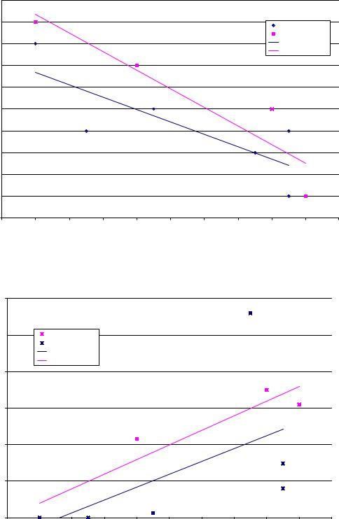
7.5 Effect of injection timing

Injection timing is one of the major factors that affects operation in regular slidercrank engines therefore it was expected to have a significant effect on the operation of the linear engine as well. Figure 59 through Figure 61 show the effect of injection timing on the operating frequency, stalling frequency, and output power respectively.

Injection timing (mm before TDC)

Figure 59. Operating frequency vs. injection timing. Advanced injection timing slightly increased the no load operating frequency. (Experimental results)

121

Injection timing (mm before TDC)

Figure 60. Stalling frequency vs. injection timing. Advanced injection timing resulted in lower stalling frequency. (Experimental results)

Injection timing (mm before TDC)

Figure 61. Power output vs. injection timing. Advancing the injection timing resulted in higher power output. (Experimental results)

122