Contrast Enhancement and Dimensionality Reduction by Principal Components

We will derive a linear transformation Ψ : R p → R p with good properties, i.e, we will find G = Ψ ( F). The resulting object g : S → R p will be an image.

Each element of each band in g = (g1, . . . , gp) will be of the form

where αi = (αi1, . . . , αip) are fixed real coefficients. Such transformation can be conveniently expressed in matrix form, i.e., g = fA, where f is the image data arranged as a mn × p matrix; any order can be used, a lexicographic one would be a good choice. The matrix A is formed by p vectors α1 . . . α p .

We are interested in finding a matrix A leading to a transformed image g with interesting properties; in particular, we would like the bands of g to be uncorrelated.

Assume the underlying distribution which characterizes F has the p × p covariance matrix Σ . Also assume this matrix is positive definite, so it can be decomposed into a matrix of eigenvectors A and a vector of eigenvalues Ξ . This means that AΣA = diag(Ξ ), where diag(Ξ ) denotes the operation that transforms a vector of dimension p into a matrix of dimension p × p with the values of Ξ in the diagonal and zero elsewhere. Now we will use the result presented in the Claim presented in page xx.

Provided we have the knowledge of Σ and, therefore, we know A and Ξ , if we make the linear transformation G = F A the covariance matrix of G is, (page xx) Cov(G) = Cov( F A) = A Cov( F) A = A Σ A = diag(Ξ ) which, by construction, is a diagonal matrix. All the elements outside the diagonal of diag(Ξ ) are zero, so all pairs of bands of G are uncorrelated. Notice that one of the few cases for which “uncorrelated” also means “independent” is the multivariate Gaussian distribution, but in most situations lack of correlation does not lead to independence.

Back to Eqs. (6.1) and (6.2), the columns of the rotation matrix A are the eigenvalues of the spectral decomposition of the covariance matrix Σ , and they are the vectors αi , 1 ≤ i ≤ p.

The elements of the diagonal matrix are Ξ = (ξ1, . . . , ξ p). They are the variances of each projection, i.e., of each band in G, and they are called the eigenvalues of the spectral decomposition of the covariance matrix Σ .

If we use the variance of each band as a measure of the information it conveys,

a single band with the most information with this criterion, one should opt for the one with highest variance.

In practice, one does not know the true, underlying covariance matrix Σ , so it has to be estimated from the data.

Listing 6.1 shows the basic steps for reading and preparing the data for the PCA. Line 1 loads the rgl library which provides high-level interfaces to OpenGL routines; it is quite convenient for the interactive visualization of, for instance, points in a

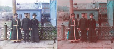
three-dimensional space. Line 2 reads the image, which is stored in a imagematrix matrix structure; the image is shown with the command issued in line 3, and the result is presented in Fig. 6.1a. Although the picture has a nice color balance, it is a good candidate for contrast enhancement by decorrelation due to the predominance of pastel tones. Figure 6.2a shows the original red, green, and blue bands. The matrix-like format, the data are stored, prevents the direct use of PCA routines, so lines 4 to 6 build a data frame with named variables, and line 7 makes them available outside the data frame. The boxplots labeled “red”, “green”, and “blue” in Fig. 6.3 present the boxplots of these three original bands; notice that they are quite “well-behaved”, with no surprising values and similar distributions. Line 18 opens an interactive plot showing the image data in 3D, each point being a pixel painted with the color it appears in the image. The user can freely choose the viewpoint and angle, and when he finds an interesting perspective, line 19 freezes the output in a PNG file, shown in Fig. 6.4a.

Listing 6.1 Reading and preparing the data

7> attach ( bands )

8> var ( bands )

Line 8 of Listing 6.1 computes and displays the covariance matrix of the original data. The reader is invited to verify that the formation content in each band, as measured by the variance, would lead us to choose the green band. It explains approximately 35 % of the total variance, while the blue and red bands carry 34 and 31 %, respectively. Line 13 calculates and exhibits the correlation matrix. It is noticeable how strong it is among all bands; it ranges between 0.91 (red and blue bands) and 0.97 (the other two pairs of bands). This linear correlation will be reduced to zero by the principal component transformation.

Line 1 of Listing 6.2 performs the Principal Components transformation. The scale and center options are the default, but in the code we stress that the data has to be centered and scaled prior to the transformation. It produces a structure, stored in pca\_image, with a number of results whose summary is displayed with the command shown in line 2.

Line 8 of Listing 6.2 assigns and displays the rotation matrix, i.e., the eigenvectors which perform the transformation. Line 13 shows that this is an orthonormal matrix: the product with its transpose is the identity matrix (with negligible errors due to the numerical representation of the data with finite precision).

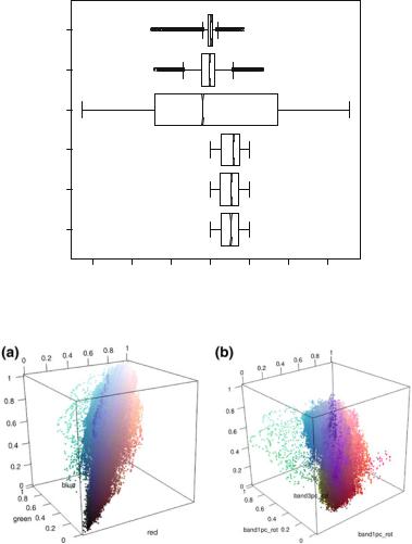
Line 21 of Listing 6.2 produces Fig. 6.3. The boxplots labeled “PC1”, “PC2”, and “PC3” describe the principal component data; technically, they are not bands since there are values outside the [0, 1] interval. Notice that the second and third principal components data are much more concentrated than the first one; c.f. line 5

(a)

(b)

(c)

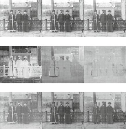
Fig. 6.2 Original and transformed bands. a Original bands. b PCA bands. c Rotated bands

of Listing 6.2 for the standard deviation of each component. Once these data have been scaled, they are shown in the form of image bands in Fig. 6.2b.

The first principal component band (Fig. 6.2b, left) looks like the negative of any of the original bands. This can be explained by the fact that the first eigenvector of the transformation (first column of lines 10, 11 and 12 of Listing 6.2) are approximately equal, and all negative. Since the PCA matrix decomposition is invariant to changes of sign applied to all the components of each eigenvector, this means that most of the information is stored in the mean of the three original bands; in fact, as presented in line 7, the first principal component explains approximately 96.77 % of the total variance conveyed in the data. The amount of information contained in the other two principal components is drastically reduced: 2.87 and 0.35 %, respectively. The original bands, ordered by the variance, explained 35, 34, and 31 %, so discarding the two least informative would have led to loosing approximately 65 % of the

Fig. 6.3 Boxplots of the original (three from bottom to top) and transformed bands

Fig. 6.4 3D visualization of pixels before and after contrast enhancement by decorrelation a Original bands. b Transformed bands

information, while doing the same with the transformed data would have discarded only about 3 %.

The results presented in line 6 of Listing 6.2 suggest one of the most important applications of the Principal Components transformation, namely, dimensionality reduction. When faced with the problem of choosing the linear transformation which conveys most of the variance (which can be understood as a measure of information content in some applications), the best choice is the first principal component. This procedure is of particular interest when dealing with remote sensing imagery, where

the number of bands range from 7 to 250, and reducing the data dimensionality may lead to faster classification algorithms with negligible loss of information.

Listing 6.3 proceeds with the principal component analysis. We will use a stretch function, as the one defined in Eq. (5.1) and implemented in lines 1–8 of Listing 5.5 (page xx). In all following cases, the minimum and the maximum output values will be 0 and 1, respectively, so, for the sake of brevity, we will refer to this function as map01.

Listing 6.3 Applying contrast enhancement by decorrelation

16plot ( imagematrix ( image _ pc ))

17plot3d ( result , pch =19 ,

18col = rgb ( band1pc _rot , band2pc _rot , band3pc _ rot ))

The principal component bands have already been rotated, i.e., the data have been projected onto the axes along which there is most variation. Lines 2 and 3 stretch these data, and they now tend to fill the new data space… but this is not the original color space, so the hues are not preserved. Since we want to preserve the colors to some extent, we have to subject the stretched data to the inverse rotation. We already know that the inverse rotation is the transpose of the forward rotation (recall the result of line 13 from Listing 6.2); this is performed in line 6 (notice the as.matrix cast to the data frame structure). Nothing grants that after the inverse rotation the data lie within the [0, 1]3 color space, so a new stretch is applied to each band independently while forming a new data frame; cf. lines 8–10 of Listing 6.3. Lines 13 and 14 transform this data frame into an image, which are subsequently plotted (line 16) and seen as points in the color space (lines 17 and 18). The results are shown in Figs. 6.1b and 6.4b, respectively.

It is interesting to compare the original and final bands. Notice that the former (Fig. 6.2a) are alike; only a very careful inspection reveals differences among them. The latter (Fig. 6.2c) exhibits variations which reflect on the more saturated colors. This is also clear comparing the 3D representation of the data, namely, Fig. 6.4a and b. The points in the latter span a bigger volume within the available color space and, as they lie further from the main diagonal, they produce more saturated colors.

Further reading on this subject is the books by Johnson and Wichern (1992); Jolliffe (2004); Krzanowski (1988, 1995); Krzanowski and Marriott (1995) and

Mardia, Kent and Bibbi (1982). The work by Muirhead (1982) is an authoritative reference for the most theoretical aspects of multivariate statistical analysis.

References

Jackson, J. E. (2003). A user’s guide to principal components. Hoboken: Wiley.

Johnson, R., & Wichern, D. (1992). Applied multivariate statistical analysis. Nueva Jersey: Prentice Hall.

Jolliffe, I. T. (2004). Principal component analysis (2nd ed.). New York: Springer.

Krzanowski, W. J. (1988). Principles of multivariate analysys: A user’s perspective, Oxford Statistical Science Series. Oxford: Claredon Press.

Krzanowski, W. J. (1995). Recent advances in descriptive multivariate analysis: Royal statistical society lecture note series (Vol. 2). Oxford: Claredon Press.

Krzanowski, W. J., & Marriott, F. H. (1995). multivariate analysis: Classification. London: Arnold. Mardia, K. V., Kent, J. T., & Bibbi, J. M. (1982). Multivariate analysis. Londres: Academic Press. Muirhead, R. J. (1982). Aspects of multivariate statistical theory: Wiley series in probability and

mathematical statistics. New York: Wiley.