Contrast Manipulation

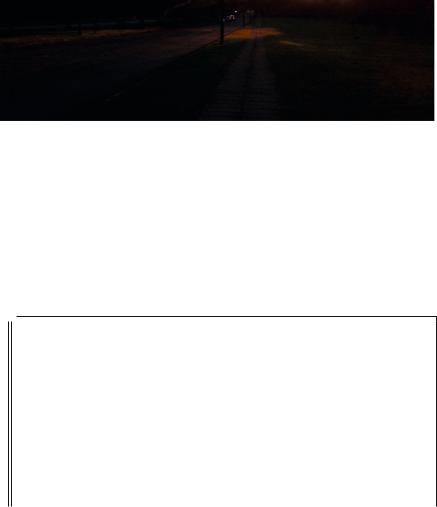
Fig. 4.1 Example image 1

using g(s) = v( f (s)) for each coordinate. In the case of color images the operation is applied for each band of the image, unless we specify another way during the text.

The image shown in Fig. 4.1 will be the example image used for all the operations presented in this chapter.

At first sight the image does not seem to have a good quality. So, before we continue, let us analyze the data of the image to search for some properties in the data that reflect this low quality. Observe Listing 4.1 presented below.

Listing 4.1 Reading the example image 1 and making basic statistical analysis

4+ red = as . vector ( image [ , ,1]) ,

5+ green = as . vector ( image [ , ,2]) ,

6+ blue = as . vector ( image [ , ,3]))

7> summary ( image . data )

Line 2 in Listing 4.1 reads the image presented in Fig. 4.1. Line 3 transforms each band of the image in a vector, and the three vectors are stored as a dataframe. In doing so, the image is now a collection of observations in [0, 1]3, i.e., without its spatial properties. In line 7, the command summary treats each vector of image.data separately and it returns a description: the minimum and maximum values, the three quantiles: the inferior, the median, the superior and the mean.

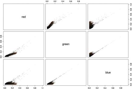
The command attach used in line 1 of Listing 4.2 makes the variables in image.data available for use through their names (red, green and blue). Line 2 draws pairs diagram, where each color represents each band of the image as illustrated in Fig. 4.2.

The diagram in Fig. 4.2 shows that the red and green bands are more strongly associated with each other than with the blue band. The graphic also shows that the

Fig. 4.2 Pairs diagram of the example image showing the correlation between each pair of bands

image has a high quantity of low saturated colors, which are closer to the diagonal that puts together the black and white colors and where the dark shades are predominant.

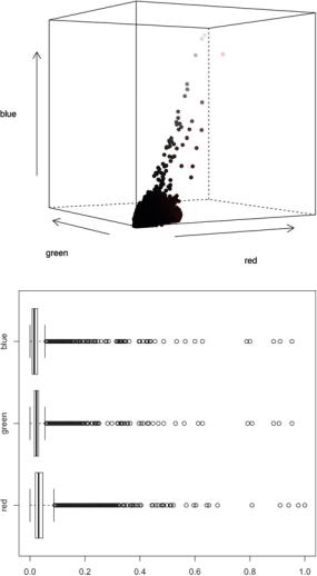
The simultaneous visualization of the cloud of values in 3D can be created in R using the library lattice, as shown in line 4 of Listing 4.2, along with the function cloud provided by this library (line 5). The created graphic is presented in Fig. 4.3.

In this figure, we notice that a high amount of values are clustered close to the diagonal that goes from the black color to the white color, and consequently, the image had low saturated colors. This effect can attenuate with the techniques of contrast improvement that will be presented later in this chapter. The reader is referred to the books by Jain (1989), Gonzalez and Woods (1992) for more details in contrast

Fig. 4.3 3D perspective of the values of three bands of the example image

Fig. 4.4 Boxplot of the bands of the example image, where it observed the misdistribution of the values for the three bands

manipulation, and to the books by Murrell (2006), Rizzo (2007) for graphics production and statistical computing in R.

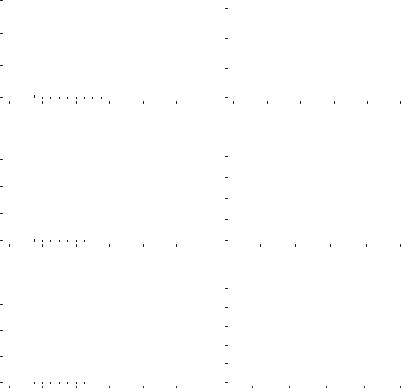
Finally, we can build a boxplot and the histogram of each band as shown in lines 7 and 9 of Listing 4.2 (only for the red band). The generated graphics are presented in Figs. 4.4 and 4.5.

The boxplot reveals that the values for the three bands are not well distributed and they are more concentrated to the left of the scale (low values), justifying the dark appearance of the image. These observations can be also seen in the histograms of the three bands in Fig. 4.5 (left column).

Fig. 4.5 Histogram of the bands of the original image (left) and of the equalized image (right)

4.1 Brightness and Contrast

For any two real numbers α and β, the pointwise operations “change of scale by α” and “addition of the value β” are defined as Sα ( f ) = α f and Tβ ( f ) = f + β, respectively, where the former is the product of scalars in each coordinate and the latter is the sum of scalars in each coordinate. The transformation Ψ is “linear” if Ψ (α f + β) = αΨ ( f ) + β for all real numbers α and β and any image f . The linear transformations can be visualized as lines in the space ( f (s), g(s)). The transformation is “linear by parts” if exists a partition of K such that for each element of the partition, the transformation is linear. An example of a linear by parts transformation for real images is g(s) = | f (s)|.

Listing 4.3 show how to apply the operations of change of scale by α and addition of the value β to the example image 1.

7> plot ( imagematrix ( image1 ))

8> plot ( imagematrix ( image2 ))

9> plot ( imagematrix ( image3 ))

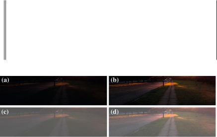
Fig. 4.6 Results after applying the transformations of change of scale by alpha, addition of the value beta, and the two former operations at the same time. a Original image. b Change of scale by 3 (contrast). c Addition of the value 0.3 (brightness). d Change of brightness and contrast

Lines 2 and 3 define the values α and β. Lines 4, 5 and 6 perform the transformation of scale, addition of value, and the two former operations at the same time, respectively. Figure 4.6 shows the result after applying the operations.

As observed in Fig. 4.6, these operations result in brightness and contrast changes in an image where the values α and β are defined by the user. However, it is not always possible to find a pair of values capable to produce an ideal result. Consequently, it is necessary to define a metric to guide the search of these values, as the variance (a contrast measure) or entropy (an information measure).

4.2 Digital Negative

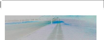
Another simple pointwise operator is the digital negative, which can be defined as: Ψs ( f (s)) = 255 − f (s) for all s S. Listing 4.4 presents a simple R code that applies this operation on the image of Fig. 4.6d. Line 1 applies the negative operator to the image resulted from line 6 of Listing 4.3 and line 2 plots the result. The values are subtracted from 1 and not from 255 because of the internal conversion applied by the software, so the values are between 0 and 1.

Figure 4.7 presents the result after applying the negative operator.

Fig. 4.8 Result after linear contrast stretch. a Original image. b Image with stretched histogram

Listing 4.5 Implementing the linear stretching operator and applying it to the example image 1 in R

possible value of K. In an opposite situation, we would have an image with a unique value, i.e., with no visual information. At first, this image with good gradation of gray levels would have a nearly normal histogram, and events with this type of histogram usually comes from random variables with uniform distribution.

Some elements of statistics defined in the previous chapter are used here to justify the technique of histogram equalization. The Theorem 1.1, for which the proof is presented in Bustos and Frery (1992), gives the theoretical support for the transformation we are looking for. The aim of the desired operation is to obtain the most uniform histogram possible. In order to achieve that, we can model the observed values as events, i.e., as occurrences of the random variable X. As we do not know

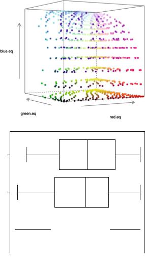
Fig. 4.10 Perspective of values of the equalized example image 1

Fig. 4.11 Boxplot of the bands of the equalized image

green blue

After the equalization process we can remake the same graphics presented in the previous section for the equalized image. Figure 4.10 shows how the values of the equalized image occupy the space. Comparing it with Fig. 4.3, the equalization improves the occupation of the color space and also moves away the colors from the main diagonal of the cube. Similarly, the boxplot of the equalized image shows that the values for each band are more uniformly distributed (see Fig. 4.11). Finally, the histogram of the bands of the equalized images are presented along with the original histograms in Fig. 4.5 (right column).

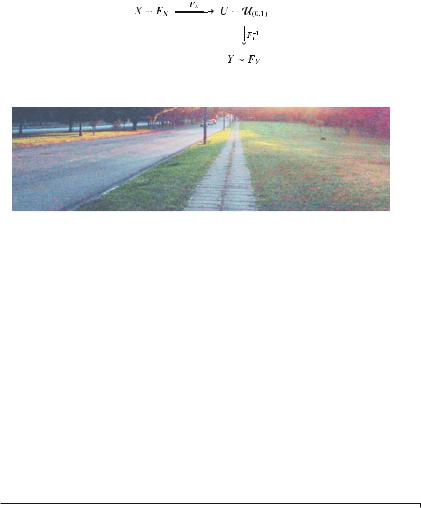
Theorem 1.1 allows the transformation of any continuous random variable into another random variable with uniform distribution inside the interval (0, 1). Theorem

Fig. 4.12 Diagram of transformation of random variables

Fig. 4.13 Example image 2 with histograms β(5, 5)

1.2 uses this result to provide an extremely efficient tool for modeling, and it comes to be one of the pillars of the stochastic simulation.

These two theorems can be seen as sets, as presented in the diagram of Fig. 4.12. It is possible, with these theorems, to transform the random variable X that follows the distribution characterized by the cumulative distribution function FX into the random variable Y that follows the distribution characterized by the cumulative distribution function FY using the transformation Y = FY−1(FX ( X)). This composition of transformations allows us to specify the histogram of an image.

In the following, we illustrate how to specify the histogram with the beta distribution (Definition 1.6). We have already seen this density for different values of the parameters a and b in Fig. 2.2a. We can produce an image with histograms following the density β(5, 5). The variables red.eq, green.eq, and blue.eq, which store the equalized bands, will be used as presented in Listing 4.7.

Listing 4.7 Producing an image with histogram specified by the density β(5, 5)

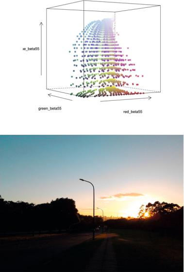
Figure 4.13 shows the result. We can notice the typical effect of a beta density with soft tails and centralized mode: the pastel shades. Using again the visualization in perspective, Fig. 4.14 shows the distribution of values of the image with the specified histogram.

Fig. 4.14 Perspective of values of the example image 1 with histograms β(5, 5)

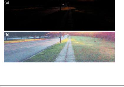
Fig. 4.15 Example image 2

The histogram equalization process presented before was applied at one time to the whole image. What if we want to equalize just part of the histogram? This would be the case when we have just one part of the image with dark colors. Let us take a look at the image in Fig. 4.15. Looking carefully to this image, we can notice that there is a clustered set of pixels with high saturated colors. This information can be inferred from the histograms of each band presented in Fig. 4.16 (left column). It

References

Bustos, O. H., & Frery, A. C. (1992). Simulação estocástica: teoria e algoritmos (versão completa), Monografias de Matemática, 49. Rio de Janeiro, RJ: CNPq/IMPA.
Coltuc, D., Bolon, P. & Chassery, J.-M. (2006). Exact histogram specification. IEEE Transactions on Image Processing, 15(5), 1143–1152. http://dblp.uni-trier.de/db/journals/tip/tip15.html# ColtucBC06
Gonzales, R., & Fittes, B. (1977). Gray-level transformations for interactive image enhancement. Mechanism and Machine Theory, 12(1), 111–122. URL http://www.sciencedirect.com/science/ article/pii/0094114X77900623, Special Issue: Robots and Manipulator Systems.
Gonzalez, R. C., & Woods, R. E. (1992). Digital Image Processing. MA: Addison-Wesley. Hummel, R. A. (1975). Histogram modification techniques. Computer Graphics and Image Process-
ing, 4(3), 209–224. URL http://www.sciencedirect.com/science/article/pii/0146664X7590009X Jain, A. K. (1989). Fundamentals of Digital Image Processing. Englewood Cliffs: Prentice-Hall
International Editions.
Murrell, P. (2006). R Graphics. Boca Raton: Chapman & Hall.
Rizzo, M. L. (2007). Statistical Computing with R. Boca Raton: Chapman & Hall/CRC.
Stark, J. A. (2000). Adaptive image contrast enhancement using generalizations of histogram equalization. IEEE Transactions on Image Processing, 9, 889–896.
Zhu, H., Chan, F. H. & Lam, F. (1999). Image contrast enhancement by constrained local histogram equalization. Computer Vision and Image Understanding, 73(2), 281–290. http://www. sciencedirect.com/science/article/pii/S1077314298907238