

Chapter 3
Reading and Writing Images with R: Generating High Quality Output
Either write something worth reading or do something worth writing.
Benjamin Franklin
We start this chapter explaining what is the core R graphics engine and how it works. A specific package provides the engine, called grDevices, which is available by default along with the standard installation of R and it is already loaded in each R session. This package provides the necessary tools for the output of graphics in different formats and also for defining graphic parameters as resolution, color, size, and fonts.
The usual process inside an R session, when an user is about to start working with an image, can be basically summarized in three steps: reading the input image, processing it, and writing the output image. The reading process will import the image as a data structure that can be manipulated inside an R session. In addition, R must be capable of rendering the imported image, such that its original aspect ratio should be maintained and also that it could be drawn relatively to the coordinate system of an R plot. In the following, the main functions used for graphics input and output are presented, both for the vector and the raster formats presented in the previous chapter.
3.1 Reading Images
3.1.1 Vector Formats
There is one package that provides a function to read vector format images, which is called grImport (Murrell 2009). As explained in the previous chapter, images in vector formats are represented geometrically. Consequently, when a vector image is
A. C. Frery and T. Perciano, Introduction to Image Processing Using R, |
31 |
SpringerBriefs in Computer Science, DOI: 10.1007/978-1-4471-4950-7_3, © Alejandro C. Frery 2013

32 |
3 Reading and Writing Images with R: Generating High Quality Output |
imported to R it is represented by a set of paths, differently from raster images that are usually represented by matrices of values. A restriction about the package is that only images in PostScript format can be read. However, there are softwares that can be used to convert images in other formats as PDF and SVG to PS, like Inkscape for instance (Bah 2011). Listing 3.1 presents a sequence of R functions that can be used to read a PostScript image.
Listing 3.1 Example of an R code that reads a vector image using the grImport package
1> library ( grImport )
2> PostScriptTrace (" Draw . ps ")
3 |
> |
draw = readPicture (" Draw . ps . xml ") |
||
4 |
> |
grid . picture ( draw ) |
||
|
|
|
||
|
|
|
|
|
|
|
|
||
|
|
|
|
|
|
|
|
|
|
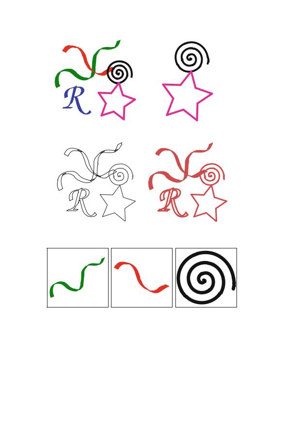
Line 1 of Listing 3.1 loads the grImport package. The PostScriptTrace function is used in Line 2 to convert the PostScript image, whose file name is passed as a parameter, into an XML document describing the contents of the image that will be read into R. The XML document is created with the same name as the image file, appending the .xml extension, in the same file path. So, in this example, Draw.ps.xml. In line 3, the ReadPicture function is used to read the XML document created previously, which creates a “Picture” object, draw. Finally, in line 4, the grid.picture function creates a grid graphical object representing the image as presented in Fig. 3.1a.
Other functions provided by the grImport package deal with the manipulation of the paths of the image. Once the image is imported inside R, the user can deal with each path separately. Let us start with a simple example, considering our “draw”. This image is composed by five paths: the green strip, the red strip, the black spiral, the pink star, and the blue “R”. The grid.picture function can be used to plot only an interval of the set of paths, as in line 1 of Listing 3.2, where only the star and the spiral are plotted, as presented in Fig. 3.1b. In order to see each path separately, the picturePaths function can be used as in line 2. The result is presented in Fig. 3.1e Line 3 presents another option of the grid.picture function, which is to ignore the fill colors of all paths (see Fig. 3.1c).
The advantage of converting the image into an XML file is that the user can change some attributes of the paths. For instance, let us change the color of all the paths in the original image and plot again the paths. These operations are presented from line 5 to 10 and the final result is shown in Fig. 3.1d. The reader is invited to explore more complex manipulations changing attributes as position, rotations, and colors or even adding other paths directly inside the XML document.
Let us show a last example using the paths of the imported “draw” image. Suppose that one want to use a different symbol in a common R plot. As a path imported from a vector image is a symbol described by its geometrical properties, it can be used easily as any other symbol by R. Take a look at Listing 3.3 and Fig. 3.2.
3.1 Reading Images |
33 |
(a) |
(b) |
(c) |
(d) |
(e)
Fig. 3.1 Original vector image imported to R and some results manipulating the paths of the image. a Original vector image. b Paths 3 and 4 of the original image. c Original image plotted ignoring the fill colors. d Image after changing the attribute “color” of all the paths. e Paths 1, 2, and 3 plotted separately
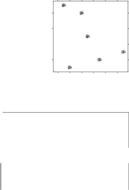
Line 1 stores all the paths into the variable called paths. In line 2, the spiral symbol is stored into the variable spiral. Lines 3 and 4 create to variables x and y to be ploted. Finally, in line 5, the xyplot is used to plot y against x using spirals
34 |
3 Reading and Writing Images with R: Generating High Quality Output |
Fig. 3.2 A common R plot whose points are represented by spirals, the symbol imported from the vector image “draw”
Changing plot symbol
8
6
y
4 

2
0 |
2 |
4 |
6 |
8 |
10 |
x
as symbols for the plot. The symbols are defined through the panel parameter, where the grid.symbols function is used to set the attributes of the spirals (size of 7 mm).
Listing 3.2 Example of some functions to manipulate vector images
1 |
> |
grid . picture ( draw [3:4]) |
|
|
2 |
> |
picturePaths ( draw [1:3] , fill =" white " ,freeScales =TRUE , |
nr =1 , |
nc =3) |
3 |
> grid . picture (draw , use . gc = FALSE ) |
|
|
|
4 |
> |
|
|
|
5 |
> |
drawRGML <- xmlParse (" Draw . ps . xml ") |
|
|
6 |
> |
xpathApply ( drawRGML ,"// path // rgb " ,’ xmlAttrs <-’, value |
= c(r |
= .8 , |
7 |
+ |
g = .3 , b = .3)) |
|
|
8 |
> saveXML ( drawRGML , " Changeddraw . ps . xml ") |
|
|
|
9 |
> |
changeddraw <- readPicture (" Changeddraw . ps . xml ") |
|
|
10 |
> |
grid . picture ( changeddraw ) |
|
|
|
|
|
|
|
|
|
|
|
|
|
|||
|
|
|
|
|
|
|
|
|
|
|
|
|
|
Listing 3.3 Example of R plot using a symbol imported from a vector image |
||||||
|
|
|
|
|
|
|
|
|
|
|
|
|
|
1 |
> |
paths <- explodePaths ( draw ) |
||||
2 |
> |
spiral <- paths [3] |
||||
3 |
> |
x |
= c (1 ,2 ,7 ,4 ,5 ,0 ,11) |
|||
4 |
> |
y |
= c (9 ,1 ,2 ,8 ,5 ,4 ,3) |
|||
5 |
> |
xyplot (y ~ x , main =" Changing plot symbol ", |
||||
6 |
+ |
panel = function (x,y ,...) { |
||||
7+ grid . symbols ( spiral ,x,y, units =" native ",size = unit (7,"mm"))
8+ })
|
|
|
|
||
|
|
|
|
|
|

3.1 Reading Images |
35 |
3.1.2 Raster Formats
Some R packages provide useful functions for reading images in raster formats. Six packages and their respective functions will be explored here: pixmap, png, rtiff, ReadImages, EBImage, and bmp. Listing 3.4 presents how to use the ReadImages package, which provides the read.jpeg function. Line 3 loads the library, line 4 reads the image, and Line 5 displays it. Similarly, using the png package, which provides the readPNG function, it is possible to read a PNG image into R as presented in Listing 3.5. In line 3, the package is loaded. In lines 4 and 5 the image is read and displayed, respectively.
Listing 3.4 Code presenting how to read jpeg images into R
1 > # Reading jpeg images
2>
3> library ( ReadImages )
4 > draw <- read . jpeg (" Draw . jpg ")
5 > plot ( draw )
|
|
|
|
||
|
|
|
|
|
|
Listing 3.5 Code presenting how to read PNG images into R
1 > # Reading png images
2>
3> library ( png )
4 > draw <- readPNG (" Draw . png ")
5 > plot ( imagematrix ( draw ))
|
|
|
|
||
|
|
|
|
|
|
In the case of TIFF images, the rtiff package must be used, which provides the readTiff function. Listing 3.6 presents how to use the package (loaded in line 2) in order to read (line 3) and display the image (three channels together as in line 4 or each channel separately as in lines 5, 6, and 7).
Listing 3.6 Code presenting how to read tiff images into R
1 |
> |
# Reading tiff |
images |
2 |
> library ( rtiff ) |
|
|
3 |
> |
draw <- readTiff (" Draw . tiff ") |
|
4> plot ( draw )
5> plot ( draw@red )
6> plot ( draw@green )
7> plot ( draw@blue )
|
|
|
|
||
|
|
|
|
|
|
Alternatively to the packages presented before, there is the EBImage package which provides the readImage function that is capable to read JPEG, PNG, and TIFF functions. This package is more sophisticated and provides several functions for manipulating images such as cropping, filtering, and applying mathematical morphology operators. Listing 3.7 presents how to read images in the three formats above using the readImage function.

36 |
3 Reading and Writing Images with R: Generating High Quality Output |
Listing 3.7 Code presenting how to use the readImage function from EBImage to read JPG, PNG, and TIFF images
1 |
|
> |
library ( EBImage ) |
|
||
2 |
|
> |
draw <- readImage (" Draw . jpg ") |
|
||
3 |
|
> |
display ( draw ) |
|
||
4 |
|
> |
draw <- readImage (" Draw . png ") |
|
||
5 |
|
> |
display ( draw ) |
|
||
6 |
|
> |
draw <- readImage (" Draw . tiff ") |
|
||
7 |
|
> |
display ( draw ) |
|
||
|
|
|
||||
|
|
|
|
|
||
|
|
|
||||
|
|
|
|
|
|
|
|
|
|
|
|
||
Finally, Listing 3.8 presents the use of the functions provided by the bmp and pixmap packages to read BMP and bitmap images respectively. Specifically, lines 2 and 3 show an example of reading and displaying a BMP image. It is important to notice that the read.bmp function is limited to 8 bit gray-scale images and 24 bit RGB images. Lines 5 and 6 show how to read and display a PPM image. The print function is provided by the pixmap package and it presents the general description of the image as presented in line 7
Listing 3.8 Code presenting how to read BMP images into R
|
|
|
|
|
|
1 |
|
> library ( bmp ) |
2 |
|
> draw <- read . bmp (" Draw . bmp ") |
3> plot ( draw )
4> library ( pixmap )
5 > draw <- read . pnm (" Draw . ppm ")
6> plot ( draw )
7> print ( draw )
8Pixmap image
9 |
|
Type |
: pixmapRGB |
||
10 |
|
Size |
: 222 x222 |
|
|
11 |
|
Resolution |
: 1 x1 |
|
|
12 |
|
Bounding box |
: 0 0 222 |
222 |
|
|
|
|
|
||
|
|
|
|
|
|
|
|
|
|
||
|
|
|
|
|
|
|
|
|
|
|
|
3.2 Writing Images
At the beginning of this chapter we have discussed about the grDevices package. This package controls the devices where a graphic is going to be displayed. During an active R session, when a graphic function is called, a graphics window is opened. This means that R uses this window as the default device, so the user do not need to decide where to send the graphics output. However, if the user wants to print the graphic in order to use in a document for instance, a graphic device must be specified, so the graphic can be saved in a file. The usual procedure is to call a function that opens a particular graphics device. After this call, all the subsequent outputs of graphic functions are produced on this device. Finally, the device must be closed calling the dev.off function. In the following, the different devices available are presented along with specific functions for writing digital images.

3.2 Writing Images |
37 |
3.2.1 Vector Formats
There are three main devices that can be used to save vector images: postscript, pdf, and svg. Let us use the same “draw” from the previous section. Assume that we have read a vector image as presented in Listing 3.1 and we have changed the image as in Listing 3.2. Now, the image can be saved in a specific device as presented in Listing 3.9.
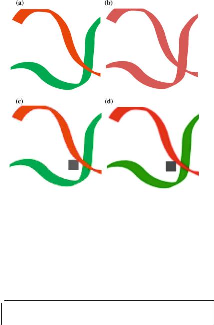
First, the image is plot as default on the graphics window inside the R session (line 1). On the other hand, in line 2, the postscript function opens an EPS file and the graphics output of the grid.picture function (line 3) is sent to this file. Finally, the file is closed in line 4. The same procedure is carried out using the other two devices as presented in lines 6 to 12. A zoomed region of the saved image is presented in Fig. 3.3b. Observe that the image still has the vector characteristics unchanged if compared with a zoomed region from the original image presented in Fig. 3.3a.
Listing 3.9 R code to save a vector image in a specific file format
|
|
|
|
|
|
1 |
|
> grid . picture (draw , use . gc = FALSE ) |
2 |
|
> postscript (" Draw _ postscript . eps ") |
3 |
|
> grid . picture (draw , use . gc = FALSE ) |
4> dev . off ()
5>
6> pdf (" Draw _ pdf . pdf " ,width =2.23 , height =2.23)
7 > grid . picture (draw , use . gc = FALSE )
8> dev . off ()
9>
10> svg (" Draw _ svg . svg " , width =2.5 , height =2.5)
11> grid . picture (draw , use . gc = FALSE )
12> dev . off ()
13>
|
|
|
|
||
|
|
|
|
|
|
3.2.2 Raster Formats
In the case of writing in raster formats, the same packages that provide the functions for reading images also provide functions for writing them. In addition, the writeJPEG function provided by the jpeg package is used. Listing 3.10 presents examples on how to use the functions for each raster format.
In lines 1 and 2 the image is read as learned in the previous section. In line 3, the values of some pixels are changed to 0.3. The changed image is written in JPEG, PNG, and TIFF in lines 5, 8, and 11, respectively. In the case of the TIFF format, the image must be converted to a data structure recognized by the writeTiff function, and this is done by the newPixmapRGB function. Similarly as the case of reading images, the EBImage package can be an alternative option to write in JPEG, PNG, and TIFF formats as presented in lines 15, 16, and 17. Finally, the image is written also in BMP (lines 19 to 21) and PPM (line 24).

38 |
3 Reading and Writing Images with R: Generating High Quality Output |
Listing 3.10 R code to save images in raster formats
1 > library ( ReadImages )
2 > draw <- read . jpeg (" Draw . jpg ")
3 > draw [80:90 ,85:95 ,] = 0.3
4> library ( jpeg )
5> writeJPEG (draw ," Draw _ jpeg . jpg" , quality =100)
6>
7> library ( png )
8> writePNG (draw ," Draw _ png . png ")
9>
10> library ( rtiff )
11> writeTiff ( newPixmapRGB ( draw [ , ,1] , draw [ , ,2] , draw [ , ,3]) ,
12+ " Draw _ tiff . tiff ")
13>
14> library ( EBImage )
15> writeImage (draw ," Draw _ jpeg2 . jpg " , type =" jpeg ")
16> writeImage (draw ," Draw _ png2 . png " , type =" png ")
17> writeImage (draw ," Draw _ tiff2 . tiff " , type =" tiff ")
18>
19> bmp (" Draw _ bmp . bmp ")
20> plot ( draw )
21> dev . off ()
22>
23> library ( pixmap )
24> write . pnm ( pixmapRGB ( draw )," Draw _ pnm . ppm ")
|
|
|
|
||
|
|
|
|
|
|
A zoomed region of the written image in raster format is presented in Fig. 3.3c. The difference between the vector and the raster formats is clear. The quality of the former is visually superior than the latter, as it is described by its geometrical shapes and it is perfectly rendered by R, differently from the raster format.
Fortunately, since version 2.11.0, R have support to render raster formats (Murrell 2011) through the grid package. This new support comes to soften the problem when rendering raster graphics, mainly for those that are intrinsically raster, i.e., graphics that are simply composed by an array of values, as the pixels of a digital image. The main advantages of using this new support is the better scaling, faster rendering and smaller graphics files. Listing 3.11 shows an example on how to use the package. In lines 1 to 3, the image is imported and displayed as usual. In line 5, the image is displayed using the grid.raster function, which provides the new rendering support. Figure 3.3d presents the resulting image saved using the grid.raster function. It can be observed the difference between the images in Figs. 3.3c, d, where the second one is clearly smoother than the first one.
Listing 3.11 Use of the grid.raster function
|
|
|
|
|
|
1 |
|
> library ( ReadImages ) |
2 |
|
> draw <- read . jpeg (" Draw . jpg ") |
3> plot ( draw )
4> library ( grid )
5> grid . raster ( draw )
|
|
|
|
||
|
|
|
|
|
|
3.2 Writing Images |
39 |
Fig. 3.3 a Original image in vector format and different output results. b Modified image saved in vector format. c Image saved in JPEG format. d Image saved in raster format using the grid.raster function
The main difference about the grid.raster function is that it uses an interpolation process when displaying the image, i.e, instead of displaying the actual pixels (squares of values), it displays an interpolation version of the values. Observe the examples presented in Listing 3.12. Line 2 creates a simple matrix of size 6 × 8 with 48 different colors. In line 3 the matrix is displayed as usual and in line 4 the same matrix is displayed using interpolation. Both results are presented in Figs. 3.4a, b, respectively.
Listing 3.12 Use of the grid.raster function
1 > library ( grid )
2 > m = matrix ( colors ()[51:98] , nrow =6)
3> grid . raster (m, interpolate =F)
4> grid . raster (m, interpolate =T)
|
|
|
|
||
|
|
|
|
|
|
40 |
3 Reading and Writing Images with R: Generating High Quality Output |
Fig. 3.4 Two examples comparing the use of the grid.raster function with 3.4a and without 3.4b interpolation
The grid package also provides the rasterImage function, which can be used to add a raster image to a usual plot. This becomes an interesting and elegant way to add graphical information to a vector plot. Observe the two examples presented in Listing 3.13. First, a simple x × y plot is built with the common plot function as presented in lines 2 to 4. Then, a matrix of size 30 × 30 is created with uniform random numbers (line 5). Finally, this matrix is added to the previous plot using the rasterImage function (line 6). The final result is shown in Fig. 3.5a. In a second example, a vector of size 50 also composed of random uniform numbers is added to the same plot (lines 8 to 10). The result is presented in Fig. 3.5b.
(a) |
|
|
|
|
|
|
(b) |
|
|
|
|
|
|
||
30 |
|
|
|
|
|
|
|
30 |
|
|
|
|
|
|
|
|
|
|
|
|
|
|
|
|
|
|
|
|
|
||
25 |
|
|
|
|
|
|
|
25 |
|
|
|
|
|
|
|
20 |
|
|
|
|
|
|
|
20 |
|
|
|
|
|
|
|
y 15 |
|
|
|
|
|
|
|
y 15 |
|
|
|
|
|
|
|
10 |
|
|
|
|
|
|
|
10 |
|
|
|
|
|
|
|
5 |
|
|
|
|
|
|
|
5 |
|
|
|
|
|
|
|
0 |
|
|
|
|
|
|
|
0 |
|
|
|
|
|
|
|
0 |
5 |
10 |
15 |
20 |
25 |
30 |
0 |
5 |
10 |
15 |
20 |
25 |
30 |
||
|
|
|
|
x |
|
|
|
|
|
|
|
x |
|
|
|
Fig. 3.5 Examples on how the rasterImage function can be used to add raster graphics in usual R plots

3.2 |
|
|
Writing Images |
41 |
||
Listing 3.13 Two examples using the rasterImage function |
|
|||||
|
|
|
|
|
|
|
|
|
|
|
|
|
|
1 |
|
> library ( grid ) |
|
|||
2 |
> |
x |
<- |
1:30 |
|
|
3 |
> |
y |
<- |
x |
|
|
4 |
|
> plot (x ,y) |
|
|||
5 |
> |
image |
<- matrix ( runif (30 * 30) , ncol =30) |
|
||
6> rasterImage ( image ,0 ,0 ,31 ,31 , interpolate =F)
7>
8> plot (x ,y)
9 |
> |
z <- runif (50) |
||
10 |
> |
rasterImage (z ,0 ,1 ,1 ,46 , angle = -48.5) |
||
|
|
|
||
|
|
|
|
|
|
|
|
||
|
|
|
|
|
|
|
|
|
|
More details about input and output in R and image formats can be found in Murrel (2011).
References
Bah, T. (2011). Inkscape: guide to a vector drawing program (4th ed.). New York: SourceForge Community Press.
Murrel, P. (2011). R Graphics (2nd ed.). Boca Raton: CRC Press.
Murrell, P. (2009). Importing vector graphics: The grImport package for R. Journal of Statistical Software, 30(4), 1–37. URL http://www.jstatsoft.org/v30/i04/
Murrell, P. (2011). Raster images in R graphics. The R Journal, 3(1), 48–54. http://journal.r-project. org/archive/2011-1/RJournal_2011-1_Murrell.pdf