

Acronyms
2D |
Two-dimensional |
3D |
Three-dimensional |
BMP |
Windows BitMap |
CMYK |
Cyan, Magenta, Yellow, Black |
EDA |
Exploratory Data Analysis |
EPS |
Encapsulated PostScript |
HSB |
Hue, Saturation, Brightness |
HSI |
Hue, Saturation, Intensity |
HSV |
Hue, Saturation, Value |
HTML |
HyperText Markup Language |
JPEG |
Joint Photographic Experts Group |
LUT |
Look up Table |
LZW |
Lempel-Ziv-Welch |
PBM |
Portable BitMap |
PCA |
Principal Component Analysis |
Portable Document Format |
|
PGM |
Portable GrayMap |
PGML |
Precision Graphics Markup Language |
Pixel |
Picture element |
PNG |
Portable Network Graphics |
PPM |
Portable PixMap |
RGB |
Red, Green, Blue |
SAR |
Synthetic Aperture Radar |
SVG |
Scalable Vectorial Graphics |
TIFF |
Tagged Image File Format |
VML |
Vector Markup Language |
W3C |
World Wide Web Consortium |
XML |
EXtensible Markup Language |
xv
Chapter 1
Definitions and Notation
Never be bullied into silence. Never allow yourself to be made a victim. Accept no one’s definition of your life; define yourself.
Harvey Fierstein
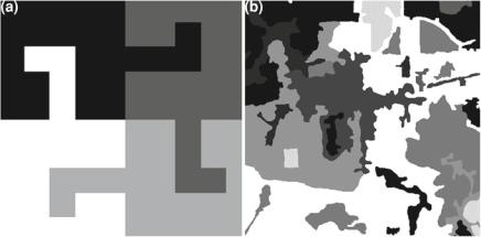
Let us start by looking at very simple cartoon images, i.e., images formed by flat areas. Images whose properties are perfectly known are usually referred to as “phantoms”. They are useful for assessing the properties of filters, segmentation, and classification algorithms, since the results can be contrasted to the ideal output. The images shown in Fig. 1.1 are phantoms, since all the relevant information they convey (the areas) is known.
The cartoon shown in Fig. 1.1a presents four disjoint regions, depicted in shades of gray ranging from white to black. It is stored as a 200 × 200 matrix of integers {1, 2, 3, 4}. It was used by Mejail et al. (2003) for the quantitative assessment of the classification of Synthetic Aperture Radar (SAR) data. The cartoon presented in Fig. 1.1b shows a hand-made map of an Amazon area. It was first employed by Frery et al. (1999) for the comparison of SAR segmentation algorithms. It is stored as a 480 × 480 matrix of integers {0, . . . , 9}. Frames are used in both cases to identify the images from the background.
What do these phantoms have in common? They have different logical sizes (the dimension of the matrices) and their values range different sets. Despite this, they are shown occupying the same physical dimension and sharing the similar colors (gray shades, in this case).
We, thus, need a formal description of the objects which will be referred to as “images” in order to be able to deal with them in an unambiguous way.
We will deal with images defined on a finite regular grid S of size m × n. Denote this support S = {1, . . . , m} × {1, . . . , n} N2. Elements of S are called sites,
coordinates or positions, and can be denoted by (i, j) S, where 1 ≤ i ≤ m is the row, and 1 ≤ j ≤ n is the column. If the coordinates are not necessary, a lexicographic order will be used to index an arbitrary element of S by s {1, . . . , mn}. Using the convention employed by R for storing data in a matrix, s = (n − 1) j +i, as illustrated
A. C. Frery and T. Perciano, Introduction to Image Processing Using R, |
1 |
SpringerBriefs in Computer Science, DOI: 10.1007/978-1-4471-4950-7_1, © Alejandro C. Frery 2013
2 |
1 Definitions and Notation |
Fig. 1.1 a Cartoon “T”, b Cartoon “Amazonia” Cartoon images
in the following code where the entries of S, that has m = 3 lines and n = 4 columns, are the values of the lexicographic order.
|
|
|
|
|
|
|
|
|
|
|
|
|
|
|
|
||
|
|
> (m |
<- matrix (1:12 , |
nrow =3)) |
|
|||
|
|
|
[ ,1] [ ,2] [ ,3] |
[ ,4] |
|
|
||
|
[1 ,] |
1 |
4 |
7 |
10 |
|
|
|
|
[2 ,] |
2 |
5 |
8 |
11 |
|
|
|
|
[3 ,] |
3 |
6 |
9 |
12 |
|
|
|
|
|
> m [11] |
|
|
|
|
|
|
|
[1] |
11 |
|
|
|
|
|
|
|
|
|
|
|
||||
|
|
|
|
|
|
|
||
|
|
|
|
|
||||
|
|
|
|
|
|
|
|
|
|
|
|
|
|
|
|
||
An image is then a function of the form f : S → K, i.e., f SK, where K the set of possible values in each position. A pixel is a pair (s, f (s)).
In many situations K has the form of a Cartesian product, i.e., K = K p, where p is called the “number of bands” and K is the set of elementary available values.
Images are subjected to storage constraints in practical applications, and, therefore, the set K is limited to computer words. Examples are the sets which can be described by one bit {0, 1} and eight bits {0, 1, . . . , 255}, either signed or unsigned integers, floating point and double precision values, and complex numbers in single and double precision.
An image is a mathematical object whose visualization has not been yet defined. A visualization function is an application ν : SK → (M, C), where M is the physical area of the monitor and C is the set of colors available in that monitor for the software which is being employed (the palette). Given an image f , ν( f ) is a set of spots in the monitor corresponding to each coordinate s S, where colors are drawn according to the values f (s). It is, therefore, clear that a binary image can be visualized in black and white, in red and blue, or in any pair of colors. . . even the same color. In this last case, the information conveyed by the image is lost in the visualization process, but can be retrieved by switching to a different set of colors.

1 Definitions and Notation |
3 |
The well-known zoom operation can be nicely understood using the visualization transformations ν1, ν2 of the binary image f : {1, . . . , 5} × {1, . . . , 10} → {0, 1}. First consider the initial visualization ν1, and assume it makes the “natural” association of (i, j) S to the physical coordinates (k, ) of the monitor: i = k and j = , and assume it paints 0 and 1 with different colors. A (2, 2) zoom is a visualization function ν2 which, while preserving the color association, maps each (i, j) S into four physical coordinates of the monitor, for instance, {(2i − 1, 2 j − 1), (2i − 1, 2 j), (2i, 2 j − 1), (2i, 2 j)}, being the only restriction the availability of physical positions. In this way, there is no need to operate directly on the data, i.e., good image processing platforms (and users) rely on visualization operations whenever possible, rather than on operations that affect the data.
In the following assume we are dealing with real-valued images of a single band, i.e., K = R. Such images are assumed to have the properties of a linear vector space (see Banon 2000 and the references therein):
• The multiplication of an image f by a scalar α R is an image g = α f SR, where g(s) = α f (s) in every s S.
•The addition of two images f1, f2 SR is an image g = f1 + f2 SR, where g(s) = f1(s) + f2(s) in every s S.
•The neutral element with respect to the addition is the image 0 SR defined as 0(s) = 0 for every s S.
These three properties allow the definition of many useful operations, among them
•The negative of the image f SR is the image g SR given by − f , i.e., the scalar product of f by −1.
•The difference between two images f1, f2 SR is the image g = f1 − f2 SR.
•The product of two images f1, f2 SR is the image g = f1 · f2 SR given by g(s) = f1(s) f2(s) for every s S.
•The ratio between f1 and f2, provided that fs (s) = 0 for every s S, g = f1/ f2 given by g(s) = f1(s)/ f2(s).
|
The assumption that S is finite allows us to define the sum of the image f SR |
||||||||
as |
f = s S f (s), and the |
mean of f as |
f |
= |
f /(mn). The inner product |
||||
|
R |
|
|
|
|
|
|||
|
S |
|
|
|
|
|
|||
between two images f1, f2 |
|
is the scalar given by f1, f2 = f1 · f2. Two |
|||||||
images are said to be orthogonal if their inner product is zero, and the norm of f SR is f = √ f, f .
Let us denote 1 the constant image 1(s) = 1 for every s S. It is immediate that 1 = 1, and that f = f, 1 .
Local operations, e.g., filters, employ the notion of neighborhood which provides a topological framework for the elements of the support S. The neighborhood of any site s S is any set of sites that does not include s, denoted ∂s S \ {s}, obeying
the symmetry relationship:
t ∂s s ∂t ,
where “\” denotes the difference between sets, i.e., A \ B = A ∩ Bc, and Bc is the complement of the set B.
4 |
1 Definitions and Notation |
Extreme cases of neighborhoods are the empty set ∂s = , and all the other sites ∂s = S \ {s} = sc. Local operations are typically defined with respect to a relatively small squared neighborhood of odd side of the form
∂ |
(i, j) = |
i |
− |
− 1 |
, i |
+ |
− 1 |
× |
j |
− |
− 1 |
, j |
+ |
− 1 |
∩ |
S |
\ |
(i, j), |
|
2 |
2 |
2 |
2 |
||||||||||||||||
|
|
|
|
|
|
(1.1) |
|||||||||||||
|
|
|
|
|
|
|
|
|
|
|
|
|
|
|
|
|
|
“small” in the sense that m and n. Notice that Eq. (1.1) holds for every (i, j) S, at the expense of reduced neighborhoods close to the edges and borders of the support.
Neighborhoods do not need to be in the form given Eq. (1.1), but this restriction will prove convenient in the forthcoming definitions.
In the following, it will be useful to restrict our attention to certain subsets of images. We will be interested, in particular, in subsets whose indexes are neighborhoods, as defined in Eq. (1.1). Assume f SR is an image, and that ∂ = {∂s : s S} is the set of neighborhoods, then f∂s : ∂s → R given by f∂s (t) = { f (t) : t ∂s , where ∂s = ∂s {s} is the closure of ∂s , is also a real valued image, defined on the grid ∂s , for every s S. We call f∂s a subimage of the image f with respect to
the window ∂s . Notice that neighborhoods, which are elements of ∂ , do not include s, whereas their closures, i.e., windows, do. The window of (maximum) odd side around site (i, j) is
∂ |
(i, j) = |
i |
− |
− 1 |
, i |
+ |
|
− 1 |
× |
j |
− |
− 1 |
, j |
+ |
|
− 1 |
∩ |
S. (1.2) |
|
2 |
2 |
2 |
2 |
||||||||||||||||
|
|
|
|
|
|
||||||||||||||
When all the interest lies on the subimage rather than on the image it comes from, it is also called a mask. In this case, the mask can be defined on the support
M |
= − |
− 1 |
, |
+ 1 |
× − |
− 1 |
, |
+ 1 |
, |
(1.3) |
|
2 |
2 |
2 |
2 |
||||||||
|
|
|
|
|
it is said to have (odd) side , and it is denoted as hM . Note that hM MR is an image defined on M.
We will use the indicator function of a set A, defined as
1 if x A,
1A(x) = 0 otherwise.
A model-based approach with many applications can be found in the book by Velho et al. (2008). The book edited by Barros de Mello et al. (2012) discusses several aspects of image processing and analysis applied to digital documents. Other important references are the works by Barrett and Myers (2004), Jain (1989), Lim (1989), Lira Chávez (2010), Gonzalez and Woods (1992) Myler and Weeks (1993), and Russ (1998) among many others.
1.1 Elements of Probability and Statistics: The Univariate Case |
5 |
1.1Elements of Probability and Statistics: The Univariate Case
Many of the images we will deal with will be simulated, in the stochastic sense. Also, many of the techniques we will discuss are based upon statistical ideas. It is therefore natural to devote this section to review basic elements of probability, statistics, and stochastic simulation. The book by Dekking et al. (2005) is a good reference for these subjects.
Probability is the branch of mathematics which deals with random experiments: phenomena over which we do not possess complete control but whose set of possible outcomes are known. These phenomena can be repeated as an arbitrary number of times under the same circumstances, and they are observable.
If Ω is the set of all possible outcomes of a random experiment, called the “sample space”, denoted by A, B outcomes, i.e., A, B Ω . A “probability” is any specification of values for outcomes Pr : Ω → R having the following properties:
1.Nonnegativity Pr( A) ≥ 0 for every A Ω .
2.An outcome is an element of the sample space Pr(Ω ) = 1.
3.Additivity Pr( A B) = Pr( A) + Pr(B) whenever A and B are disjoint, i.e., and
A ∩ B = .
Instead of working with arbitrary sets, we will transform every outcome into a set of the real line, say X : Ω → R. Such transformation, if well defined, is known as “random variable”. As possible we can know about a random variable is the probability of any possible event. Such knowledge amounts to saying that we “know the distribution” of the random variable. Among the ways we can know the distribution of the random variable X, one stems as quite convenient: the “cumulative distribution function” which is denoted and defined as
FX (t) = Pr(X ≤ t).
There are three basic types of random variables, namely discrete, continuous, and singular. We will only deal with the two former which are defined in the following:
Definition 1.1 (Discrete random variable). Any random variable which maps a finite or countable sample space is discrete.
For convenience but without loss of generality, assume X : Ω → Z. The distribution of such random variables is also characterized by the “probability vector”, that is denoted and given by
pX = . . . , (−1, Pr(X = −1)), (0, Pr(X = 0)), (1, Pr(X = 1)), . . .
=i, Pr(X = i) i Z.
It is clear that i Z Pr(X = i) = 1 by Property 2 above.
6 1 Definitions and Notation
Definition 1.2 (Continuous random variable). The random variable X is contin-
uous if exists a function h : R → R+ such that FX (t) = |
t |
−∞ h(x) dx for every |
|
t R. |
|
If h exists it is called the “density” which characterizes the distribution of X, or just “the density” of X.
Given a function Υ : R → R, the expected value of the random variable Υ (X), provided the knowledge of the distribution of X, is given by E(Υ (X)) =
R Υ (x)h X (x)dx if the random variable is continuous, and by E(Υ (X)) =
pX (x)dx otherwise, provided the integral or the sum exist. If Υ is the identity function, we have the mean or expected value E(X); if Υ (X) = E(X2) − (E(X))2 we have the variance.
In the following, we will define basic probabilistic models, i.e., distributions, which will be used in the rest of this book.
Definition 1.3 (Uniform discrete model). A random variable is said to obey the uniform discrete model with k ≥ 1 states if its distribution is characterized by the probability vector
1 |
|
1 |
|
|
1, |
|
, . . . , k, |
|
. |
|
|
|||
|
k |
k |
||
Definition 1.4 (Poisson model). The random variable X : Ω → N is said to obey the Poisson model with mean λ > 0 if the entries of its probability vector are
k, e−λ λk . k!
Definition 1.5 (Uniform continuous model). The random variable X : Ω →
[a, b], with a < b, is said to follow the uniform law on the [a, b] interval if the density which characterizes its distribution is
1
h(x; a, b) = b − a 1[a,b](x),
where 1A the indicator function of the set A.
The uniform distribution is central in probability and computational statistics. It is the foundation of the algorithms to generate occurrences of random variables of any type of distribution (see Bustos and Frery 1992 and the references therein).
Definition 1.6 (Beta model). The random variable X : Ω → [0, 1] obeys the Beta model with parameters p, q > 0 if its density is
h(x |
; |
p, q) |
= |
Γ ( p + q) |
x p−1(1 |
− |
x)q−1. |
(1.4) |
|
||||||||
|
|
Γ ( p)Γ (q) |
|
|
||||
This situation is denoted as X B( p, q).

1.1 Elements of Probability and Statistics: The Univariate Case |
7 |
If p = q = 1 the Beta distribution reduces to the uniform continuous model on the [0, 1] interval. If p > 1 and q > 1 the mode of this distribution is
q |
|
(X) |
|
|
α − 1 |
. |
|||
1/2 |
= α |
|
|||||||
|
|
+ |
β |
− |
2 |
|
|||
|
|
|
|
|
|
|
|
||
This, with the facts that its mean and variance are, respectively,
μ = E(X) = |
|
p |
|
, |
|
|
|
|
|
|
(1.5) |
p |
+ |
q |
pq |
|
|
|
|
|
|||
σ 2 = Var(X) = |
|
|
|
|
|
|
|
(1.6) |
|||
|
|
|
|
|
|
|
, |
||||
|
|
|
|
|
|
|
|
||||
( p |
+ |
q)2( p |
+ |
q |
+ |
1) |
|||||
|
|
|
|
|
|
|
|
||||
gives us a handy model for the simulation of images. Straightforward computation
yields that
μ
p = q, (1.7) 1 − μ
a handy relation for stipulating the parameters of samples with a fixed desired mean μ.
Definition 1.7 (Gaussian model). The random variable X : Ω → R is said to2obey |
|||||||
the Gaussian (often also called normal) model with mean μ R and variance σ |
> 0 |
||||||
if its density is |
|
|
|
|
|||
1 |
|
1 |
|
|
|||
h(x; μ, σ 2) = |
√ |
|
exp |
− |
|
(x − μ)2 , |
|
2σ 2 |
|
||||||
2π σ 2 |
|
||||||
√
where σ = σ 2 is known as “standard deviation”. If μ = 0 and σ 2 = 1, it is known as the standard Gaussian distribution.
The main inference techniques we will employ require the knowledge of two elements, defined in the following.
Definition 1.8 (Moment of order k). The moment of order k of the distribution D, characterized either by the probability vector pX or by the density h X is given by
mk = |
R xk h X (x)dx |
(1.8) |
mk = |
xk pX (x), |
(1.9) |
Z
respectively, if the integral or the sum exists.
The basic problem of statistical parameter estimation can be posed as follows. Consider the parametric model D(θ ), with θ Θ R p, where Θ is the parametric space of dimension p ≥ 1. Assume the random variables X = (X1, . . . , Xn ) follow this model, and they are independent. The vector x = (x1, . . . , xn ) is formed by
8 |
1 Definitions and Notation |
an observation from each of these random variables. An estimate of θ is a function θ (x) which we expect will give us an idea of the true but unobserved parameter θ . The estimator θ (X ) is a random variable. One of the most fundamental properties expected from good estimators is the consistency: limn→∞ θ (X ) → θ .
Without loss of generality, in the following we will define the two main estimation techniques only for the continuous case. The reader is referred to the book by Wassermann (2005) for more details and further references.
Definition 1.9 (Estimation by the method of moments). The estimator θ is obtained by the method of moments if it is a solution of the system of equations
f1(θ ) − mi1 |
= 0, |
(1.10) |
|
. |
|
|
. |
|
|
. |
|
f p(θ ) − mi p |
= 0, |
(1.11) |
where f1, . . . , f p are linearly independent functions, the left-hand side of Eq. (1.8), and mi1 , . . . , mi p are all different sample moments, i.e.,
1 |
n |
|
m j = |
|
X j . |
n |
||
|
|
i=1 |
Definition 1.10 (Estimation by maximum likelihood). The estimator θ is a maximum likelihood estimator if it satisfies
n
θ |
= arg |
max |
|
1 h X (Xi ; θ ), |
(1.12) |
|
θ Θ i |
= |
|||
|
|
|
|
|
where the dependence of the density on the parameter θ is explicit.
Since all densities in Eq. (1.12) are positive, we may maximize the logarithm of the product instead.
As will be seen later, R provides routines for computing maximum likelihood estimates in a wide variety of models.
Theorem 1.1 (Transformation by the cumulative distribution function itself).
Let X be a continuous random variable for which the distribution is characterized by the cumulative distribution function FX . The random variable U = FX (X) has uniform distribution in (0, 1).
Definition 1.11 (Empirical function). Consider x1, . . . , xn as occurrences of the random variables X1, . . . , Xn : Ω → [0, 1], where all of them have the same distribution characterized by the cumulative distribution function F. The empirical function, given by
1.1 Elements of Probability and Statistics: The Univariate Case |
9 |
||||
F(t) = |
1 |
#{i |
: xi |
≤ t}, |
|
|
|
||||
n |
|
||||
is an estimator of F.
The properties of the empirical function and its relationship with robust inference can be seen in the classical book of Huber (1981).
Theorem 1.2 (Transformation |
by inversion). Let U and F : R −→ [0, 1] be |
an uniform distributed random |
variable in (0, 1) and the cumulative distribu- |
tion function of a continuous random variable, respectively. The random variable Y = F−1(U ) follows the distribution characterized by F.
The proof of the Theorem 1.2 and its extension to discrete random variables can be seen in Bustos and Frery (1992).
1.2 From Phantoms to Single Band Images
We already have the necessary apparatus for simulating images. As previously stated, often times the support K of the image is a compact set. In these cases, a precise modeling prevents the use of distributions which are defined on the real numbers R, the positive numbers R+ and so on.
Consider, for instance, the situation where K = [0, 1]. Any Gaussian model for the data will assign a positive probability to events which do not belong to K and, therefore, cannot be considered as image data. In order to circumvent such issue, the data are frequently subjected to a truncation process.
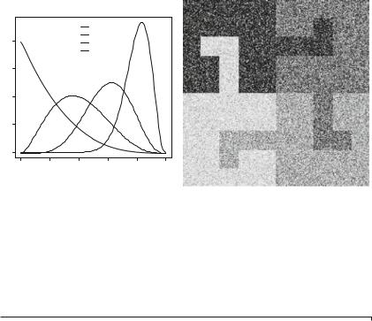
Instead of doing so, we will build images from the phantoms using the Beta model. Consider the phantom presented in Fig. 1.1a. It is composed of four areas, so we choose four equally spaced mean values in the [0, 1] interval: 0.2, 0.4, 0.6, and 0.8. Using the relation given in Eq. (1.7), and fixing q = 4, if we want observations with means μk {.2, .4, .6, .8} we have to sample from the B( pk , 4) law with pk {1, 8/3, 6, 16}. These four densities are shown in Fig. 1.2a, while the observed image under this model is shown in Fig. 1.2b.
In the following, we will see how the plot and the figure were produced in R.
R provides a number of tools related to distribution functions. They are gathered together by a prefix, indicating the type of function, and a suffix, associated to the distribution. For instance, for the Beta distribution (presented in Definition 1.6), R provides the functions dbeta (density function, as expressed in Eq. 1.4, pbeta (cumulative distribution function), qbeta(quantiles), andrbeta (simulation of Beta deviates). Instead of building our own density function, we will use the one provided by R.
The code is presented in Listing 1.1. Line 1 builds a vector with 500 equally spaced elements, starting in zero and ending in one; this will be the abscissa of all densities. Lines 2 and 3 draw the first Beta density with p = 16 and q = 4; it also
10 |
|
|
|
|
|
1 |
Definitions and Notation |
|
(a) |
|
|
|
|
(b) |
|
|
|
|
|
p = 1 |
|
|
|
|
4 |
|
|
p = 8/3 |
|
|
|
|
|
|
p = 6 |
|
|
|
|
|
|
|
|
|
|
|
|
|
|
|
|
p = 16 |
|
|
|
densities |
3 |
|
|
|
|
|
|
4) |
2 |
|
|
|
|
|
|
p, |
|
|
|
|
|
|
|
B ( |
1 |
|
|
|
|
|
|
|
|
|
|
|
|
|
|
|
0 |
|
|
|
|
|
|
|
0.0 |
0.2 |
0.4 |
0.6 |
0.8 |
1.0 |
|
|
|
|
Intensity |
|
|
|
|
Fig. 1.2 a Beta densities. b Phantom under the Beta model Four Beta densities and observed image under the Beta model
sets the labels (notice the use of the expression command). We start by this curve because it is the one which spans the largest ordinates interval. Lines 7–9 produce the legend.
Listing 1.1 Drawing Beta densities
1 |
|
|
x <- seq (0 , 1, |
length =500) |
|
|
|
|
2 |
|
|
curve ( dbeta (x , |
16 , |
4) , lty =4 , xlab =" Intensity " , |
|
||
3 |
|
|
ylab = expression ( italic (B )( italic (p), |
4) * " densities ") ) |
|
|||
4 |
|
|
curve ( dbeta (x, |
6, |
4), add =TRUE , lty =3) |
|
|
|
5 |
|
|
curve ( dbeta (x, |
8/3, 4), add =TRUE , lty =2) |
|
|
|
|
6 |
|
|
curve ( dbeta (x, |
1, |
4), add =TRUE , lty =1) |
|
|
|
7 |
|
|
legend (x="top", expression ( italic (p) == 1, italic (p) == 8/3, |
|
||||
8 |
|
|
italic (p) |
== 6, italic (p) == 16) , |
bty="n", |
|
||
9 |
|
|
lty =1:4) |
|
|
|
|
|
|
|
|
|
|
||||
|
|
|
|
|
|
|
||
|
|
|
|
|
||||
|
|
|
|
|
|
|
|
|
|
|
|
|
|
|
|
||
The example presented in Listing 1.1 is not a paradigm of economic R code. All codes presented in this book place readability in front of elegance and economy. The reader is strongly encouraged to try it, experimenting the countless possibilities the language offers.
The T phantom is available in the Timage.Rdata file. Listing 1.2 shows how to read this phantom and to produce the image shown in Fig. 1.2b. Line 1 reads the data which stores the phantom, and Line 2 checks the unique values in this matrix; they are 1, 2, 3, and 4. Line 3 makes a copy of the phantom in a new variable (TBeta) which will be the sampled image; this spares the effort to discover and set the dimensions of the output. Lines 4–7 sample from each Beta distribution the correct number of observations (200*200/4, since each class occupies exactly one fourth of the phantom), with the desired parameters. Line 8 transforms the data matrix into an image, which can be visualized with the command plot.

1.2 From Phantoms to Single Band Images |
11 |
Listing 1.2 Reading the phantom and producing the beta image
1load (" .. / Images / Timage . Rdata ")
2unique ( sort (T ))
3 |
|
TBeta <- T |
|
|
|
|
|
|
|
|
4 |
|
TBeta [ which (T == 1)] <- |
DarkestBeta <- rbeta (200 |
* 200 /4 |
, 1 |
, |
4) |
|
||
5 |
|
TBeta [ which (T == 2)] <- |
rbeta (200 * 200 /4, |
8 |
/3, 4) |
|
|
|
|
|
6 |
|
TBeta [ which (T == 3)] <- |
rbeta (200 * 200 /4, |
6 |
, 4) |
|
|
|
|
|
7 |
|
TBeta [ which (T == 4)] <- |
BrightestBeta <- |
rbeta (200 * 200 |
/4, |
|
16 , 4) |
|
||
8 |
|
plot ( imagematrix ( TBeta )) |
|
|
|
|
|
|
|
|
|
|
|
|
|
|
|
|
|
||
|
|
|
|
|
|
|
|
|
|
|
|
|
|
|
|
|
|
|
|
||
|
|
|
|
|
|
|
|
|
|
|
|
|
|
|
|
|
|
|
|
|
|
Notice that the data in the darkest and brightest areas have been stored in the variables DarkestBeta and BrightestBeta, respectively, for future use.
In this example, we worked within the [0, 1] interval, so there is no need to further transform the data to fit into the imagematrix restriction. Had we used the Gaussian distribution or any other probability law with a noncompact support, such transformation would have been mandatory, as will be seen in the next example.
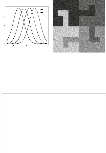
The Gaussian model presented in Definition 1.7 (p. x) is the most notorious and overall employed statistical model, mainly due to historical reason and to the fact that it has nice mathematical properties. Many image processing techniques rely on the Gaussian hypothesis. We built the image presented in Fig. 1.2b by fixing one of the parameters of the Beta distribution and choosing the desired mean; the other parameter, and the variance, are a consequence of this choice. In the following, we will use the Gaussian model to freely stipulate the mean and the variance of data in each region.
Figure 1.3 presents the Gaussian model and an image produced by it. The similarity between Figs. 1.2b and 1.3b is striking, albeit the models are quite different, as can be seen comparing Figs. 1.2a and 1.3a. This is due to the inability of the human eye to perceive statistics beyond the first moment, i.e., the mean; since the means in each region under the Beta and the Gaussian model are equal, it is quite hard to tell them apart.
As in the Beta model example, the data in the darkest and brightest areas have been stored in the variables DarkestGaussian and BrightestGaussian, respectively. Later we will see how to take samples by interactively choosing areas in an image, but direct attribution, as seen here, suffices for the moment. In the following we will analyze these data, including a fit to their models.
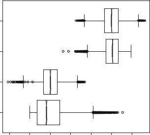
Listing 1.3 presents the descriptive analysis of the darkest and brightest areas from both the Beta and Gaussian models. First, we fix the number of decimal digits of the output to two (line 1). Second, a summary command is issued for each data set. This command produces as output the minimum, first quantile, median, mean, third quartile, and maximum values of its input. In this listing, we mix both input and output in R; the former is prefixed by the “>” symbol. It is noticeable that the means coincide in both regions, but all other quantities differ. Lines 14–16 store the four variables in a very convenient R structure: a dataframe; this is done also by fixing the name of each variable to a mnemonic pair of characters. Lines 17 and 18 produce the boxplot shown in Fig. 1.4. The option notch=TRUE adds a graphical
12 |
|
|
1 |
Definitions and Notation |
(a) |
|
|
(b) |
|
|
2.0 |
|
=0.2 |
|
|
|
|
=0.4 |
|
|
|
|
=0.6 |
|
|
|
|
=0.8 |
|
0.04) densities |
1.0 1.5 |
|
|
|
N(, |
0.5 |
|
|
|
|
0.0 |
|
|
|
|
0.0 |
0.5 |
1.0 |
|
|
|
Intensity |
|
|
Fig. 1.3 a Gaussian densities. b Phantom under the Gaussian model Four Gaussian densities and observed image under the Gaussian model
representation of the confidence interval of each median which, in this case, suggest the differences are not random. The asymmetry of the data from the dark Beta model is evident in this plot, as well as the different spread of the data around the medians. Details about this plot can be found in the book by Dekking et al. (2005).
Listing 1.3 Descriptive analysis of data from the darkest and brightest areas
1> options ( digits =2)
2> summary ( DarkestBeta )
3 |
|
|
Min . 1 st Qu . |
Median |
Mean 3 rd Qu . |
Max . |
|||
4 |
|
|
0.00 |
0.07 |
0.16 |
0.20 |
0.29 |
0.91 |
|
5 |
> |
summary ( DarkestGaussian ) |
|
|
|
|
|||
6 |
|
|
Min . 1 st Qu . |
Median |
Mean 3 rd Qu . |
Max . |
|||
7 |
|
|
-0.21 |
0.13 |
0.20 |
0.20 |
0.27 |
0.54 |
|
8 |
> |
summary ( BrightestBeta ) |
|
|
|
|
|||
9 |
|
|
Min . 1 st Qu . |
Median |
Mean 3 rd Qu . |
Max . |
|||
10 |
|
|
0.33 |
0.74 |
0.81 |
0.80 |
0.86 |
0.99 |
|
11 |
> |
summary ( BrightestGaussian ) |
|
|
|
||||
12 |
|
|
Min . 1 st Qu . |
Median |
Mean 3 rd Qu . |
Max . |
|||
13 |
|
|
0.45 |
0.73 |
0.80 |
0.80 |
0.86 |
1.13 |
|
14 |
> |
DarkestBrightest <- data . frame ( DB <- DarkestBeta , |
|||||||
15 |
|
|
DG <- DarkestGaussian , |
BB <- BrightestBeta , |
|||||
16 |
|
|
BG <- BrightestGaussian ) |
|
|
|
|||
17 |
> |
boxplot ( DarkestBrightest , |
horizontal =TRUE , notch =TRUE , |
||||||
18 |
|
|
names =c(" DB " , |
" DG " , " BB " , " BG "), xlab =" Intensities ") |
|||||
|
|
|
|
|
|
|
|
||
|
|
|
|
|
|
|
|
|
|
|
|
|
|
|
|
|
|
||
|
|
|
|
|
|
|
|
|
|
|
|
|
|
|
|
|
|
|
|
So far we made a very simple descriptive analysis of the data contained in the image shown in Fig. 1.2b, assuming that we have labels for each value, i.e., that we know the class it comes from. This descriptive analysis consisted in calling the summary function and in drawing boxplots and histograms, but Exploratory Data
1.2 From Phantoms to Single Band Images |
13 |
DB DG BB BG
−0.2 |
0.0 |
0.2 |
0.4 |
0.6 |
0.8 |
1.0 |
Intensities
Fig. 1.4 Boxplots of the darkest and brightest data from the Beta and Gaussian models
Analysis—EDA, originated by Tuckey (1973), is a well established and growing speciality of statistics which offers much more.
EDA lets the data speak for themselves, without strong assumptions about the underlying distributions and relationships among them. It is more a collection of tools, both graphical and quantitative, than a formal approach. EDA practitioners are guided by intuition and results, rather than by established recipes. Every sound data analysis in image processing (and in any other area) should be preceded careful and as exhaustive as possible EDA. Unfortunately, this is seldom seen in the literature.
One step further consists in assuming a parametric model and estimating the parameters using the available data. Assume the data came from the Beta distribution; the code presented in Listing 1.4 shows how to estimate the parameters by maximum likelihood. Line 1 reads the MASS library which provides the fitdistr function. This function fits univariate data to parametric models, offering flexibility to fix or constraint the parameters. The model can be one of a comprehensive list of predefined distributions (which includes the Beta, the Gaussian and other important probability laws), or it can be specified through a density or probability function. It requires a starting point for the search of the estimates, which is provided by means of a named list (see Line 2). Upon a successful call, the function fitdistr returns an R object containing the parameter estimates, their estimated standard errors, the estimated variance-covariance matrix, the value of the log-likelihood function at the estimates; only the first two are shown by default, as seen in lines 5 and 6. Lines 7 and 8 extract
14 |
|
|
1 Definitions and Notation |
|
4 |
|
|
|
|
|
Density |
3 |
|
|
|
|
Empirical |
2 |
|
|
|
|
Proportions and |
1 |
|
|
|
|
|
0 |
|
|
|
|
|
0.0 |
0.2 |
0.4 |
0.6 |
0.8 |
|
|
|
Intensities |
|
|
Fig. 1.5 Histogram and empirical Beta density for the darkest region of the Beta image
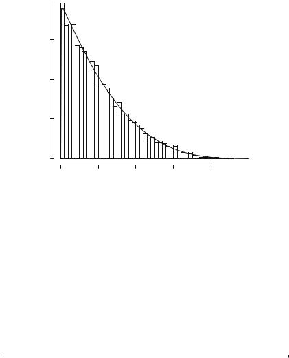
the estimates from the object and assign them to mnemonic variables. Notice that the estimates ( p, q) = (1.017, 4.090) and the true values ( p, q) = (1, 4) are very close, and even closer when we notice that the observed bias (the difference between the true and estimated values) is within less than two observed standard deviations. The estimated parameters will be now used to draw the empirical (estimated) density over the histogram. This will serve as a visual assessment of the quality of the model. Lines 9–11 compute and plot the histogram of the data using the Friedman-Diakonis (breaks=“FD”) algorithm for computing the points at which the breaks are. Line 12 computes and adds the empirical density to the proportions histogram, showing how similar they are. The result of running this piece of code is shown in Fig. 1.5.
Listing 1.4 Maximum likelihood estimation of the parameters of the Beta distribution
1 |
|
> |
library ( MASS ) |
|
||||
2 |
|
> |
( DarkestParameters <- fitdistr ( DarkestBeta , " beta " , |
|
||||
3 |
|
|
|
|
start = list ( shape1 =1 , shape2 =1))) |
|
||
4 |
|
|
|
shape1 |
shape2 |
|
||
5 |
|
|
|
1.017 |
4.090 |
|
|
|
6 |
|
|
|
(0.013) (0.061) |
|
|
||
7 |
|
> |
pd |
<- |
DarkestParameters $ estimate [1] |
|
||
8 |
|
> |
qd |
<- |
DarkestParameters $ estimate [2] |
|
||
9 |
|
> |
hist ( DarkestBeta , xlab =" Intensities " , |
|
||||
10 |
|
|
|
|
ylab =" Proportions and Empirical Density ", |
|
||
11 |
|
|
|
|
main ="", breaks ="FD", probability = TRUE ) |
|
||
12 |
|
> |
curve ( dbeta (x, pd , qd), from =0, to =1, add =TRUE , n =500) |
|
||||
|
|
|
|
|
||||
|
|
|
|
|
|
|
||
|
|
|
|
|
||||
|
|
|
|
|
|
|
|
|
|
|
|
|
|
|
|
||
The reader is invited to repeat this analysis using the data from the brightest region.
1.3 Multivariate Statistics |
15 |
1.3 Multivariate Statistics
We have dealt with images with a single band, but multiband imagery is also treated in this book (these concepts are defined in the next section). While, as already seen, the former can be described with univariate random variables, the latter require multivariate models.
Definition 1.12 (Multivariate random variables). A random vector is a function
X : Ω → Rm such that each component is a random variable.
The distribution of the random vector X = (X1, . . . , Xm ) is characterized by the multivariate cumulative distribution function:
FX (x1, . . . , xm ) = Pr(X1 ≤ x1, . . . , Xm ≤ xm ).
If there is a function hX such that
x1 |
|
xm |
FX (x1, . . . , xm ) = |
. . . |
hX (t1, . . . , tm )dt1 . . . dtm , |
−∞ |
|
−∞ |
then the random vector X is said to be continuous, and hX is the density which characterizes its distribution. Although there are plenty of discrete multivariate distributions (c.f. the book by Johnson et al. 1997 and the references therein), for the purposes of this book it will suffice to consider continuous random variables. In particular, the only continuous multivariate distribution we will employ in this book is the Gaussian law. More continuous multivariate distributions can be found in the book by Kotz et al. (2000).
We need new definitions of the mean and the variance when dealing with multivariate distributions. The vector of means (or mean vector) of X : Ω → Rm is
E(X ) = (E(X1), . . . , E(Xm )),
provided it exists. The covariance matrix of the random vector is Σ = (σi j )1≤i, j≤m , the m × m matrix whose elements are the covariances σi, j = Cov(Xi , X j ), provided they exist. The diagonal elements (σii )1≤i≤m are the variances σii = Var(Xi ).
Provided all the elements of the covariance matrix Σ exist, the correlation matrix= ( )1≤i j≤m is given by the m × m correlation coefficients
i j = |
|
Cov(Xi , X j ) |
; |
|
|
||
Var(Xi )Var(X j ) |
clearly, ii = 1 for every 1 ≤ i ≤ m. If Σ is positive definite, then −1 < i j < 1, and if i j = 0 we say that Xi and X j are uncorrelated.
Definition 1.13 [(Proper) multivariate Gaussian distribution]. Consider the vector μ Rm and the positive definite matrix Σ . The random vector X : Ω → Rm

16 |
1 Definitions and Notation |
obeys the m-variate Gaussian distribution if the density which characterizes its distribution is
fX (x) = |
|
1 |
√ |
|
exp − |
1 |
(x − μ) Σ −1(x − μ) |
(1.13) |
|
|
m/2 |
|
2 |
||||||
(2π ) |
|Σ | |
||||||||
|
|
|
|
|
|
|
where denotes transposition, and |Σ | is the determinant of the matrix Σ . The vector μ is the vector of means, and Σ is the covariance matrix.
The maximum likelihood estimators of μ and Σ based on a sample of size n of independent and identically distributed multivariate Gaussian random variables X1, . . . , Xn are, respectively
1 |
n |
1 |
n |
|
||
μ = |
|
|
Xi , and Σ = |
|
(Xi − μ) (Xi − μ). |
(1.14) |
n |
i=1 |
n |
||||
|
|
|
|
i=1 |
|
|
The multivariate Gaussian distribution is a commodity of image processing software: most algorithms assume it holds, and are therefore based on procedure which produce optimal results under this assumption. The assumption itself is seldom checked in practice.
A practical consequence of assuming the multivariate Gaussian model for the random vector X : Ω → Rm is that if it holds, then every component (Xi )1≤i≤m obeys a Gaussian distribution. R provides a number of routines for checking the goodness- of-fit to arbitrary distributions (among them the well-known χ 2 and KolmogorovSmirnov tests), but also a specialized one: the Shapiro-Wilk test (Cohen and Cohen 2008). Graphical tools as, for instance, Quantile–Quantile (QQ) plots are also handy tools for checking the quality of a model.
The following result will be useful when dealing with principal component analysis in Chap. 6.
Claim [Linear transformation of multivariate random variables] Assume X : Ω → Rm is an m-variate random variable with covariance matrix Σ . Let A be an m × m matrix. The covariance matrix of the random variable AX is AΣ A .
1.4 Multiband Images
We conclude this chapter using the cartoon model presented in Fig. 1.1b. In the same way we previously “filled” each area of the cartoon model shown in Fig. 1.1a with samples from univariate distributions, producing the images shown in Figs. 1.2b and 1.3b, we will replace each class in the Amazonia cartoon model by a sample from a multivariate Gaussian random variable whose parameters are constant along each of the ten classes.

1.4 Multiband Images |
17 |
Let us start by defining ten mean vectors: three in red, three in green, and three in blue shades, plus a gray tone, detailed as follows:
0.50 |
0.75 |
0.75 |
|
μR1 = 0.25 , μR2 = 0.50 , μR3 = 0.50 |
, |
||
0.25 |
0.25 |
0.50 |
|
0.25 |
0.25 |
0.25 |
|
μG1 = 0.50 , μG2 = 0.75 , μG3 = 0.75 , |
|||
0.25 |
0.25 |
0.50 |
|
0.25 |
0.25 |
0.50 |
|
μB1 = 0.25 , μB2 = 0.50 , μB3 = 0.50 , |
|||
0.50 |
0.75 |
0.75 |
|
and μG (0.50 0.50 0.50) , respectively. The command for defining μR1 is just Red1 <- c(.50, .25, .25); the others follow immediately.
Also ten covariance matrices were chosen to specify the distribution of the data in each class. In order to avoid tedious typing, which is also prone to errors, we defined a function which accepts the values of three standard deviations and three correlation coefficients, and produces a covariance matrix as output. This function is presented in Listing 1.5.
Listing 1.5 Function which returns a covariance matrix based on three standard deviations and three correlation coefficients
1 |
BuildCovMatrix |
<- function (s1 , s2 , |
s3 , r12 , r13 , r23 ) { |
|||
2 |
|
|
|
|
|
|
3 |
CovMatrix |
<- |
matrix ( rep (0 , |
9) , nrow =3 , ncol =3) |
||
4 |
|
|
|
|
|
|
5 |
variances |
<- |
c( s1 ^2 , s2 ^2 , |
s3 ^2) |
|
|
6 |
|
|
|
|
|
|
7 |
for (i in |
1:3) |
|
CovMatrix [i ,i] <- |
variances [i] |
|
8 |
|
|
|
|
|
|
9 |
CovMatrix [1 ,2] |
<- CovMatrix [2 ,1] |
<- r12 * s1 * s2 |
|||
10 |
CovMatrix [1 ,3] |
<- CovMatrix [3 ,1] |
<- r13 * s1 * s3 |
|||
11 |
CovMatrix [2 ,3] |
<- CovMatrix [3 ,2] |
<- r23 * s2 * s3 |
|||
12 |
|
|
|
|
|
|
13return ( CovMatrix )
14}
|
|
|
|
||
|
|
|
|
|
|
Line 3 creates a new matrix of size 3 × 3 filled with zeroes. Line 5 defines the variances as the square of each standard deviation passed in the input. Line 7 assigns each variance to an element in the diagonal of the matrix, while lines 9–11 compute the off-diagonal elements.

18 |
1 Definitions and Notation |
The commands presented in Listing 1.6 instantiate the ten covariance matrices employed in our simulation experiment. They are combinations of two values of standard deviation (intense 0.1 and weak 0.07) and to levels of correlation (intense 0.9 and weak 0.3)
Listing 1.6 Defining covariance matrices
1 |
|
> |
si <- 0.1 |
|
||
2 |
|
> |
sw <- 0.07 |
|
||
3 |
|
> |
ri <- 0.9 |
|
||
4 |
|
> |
rw <- 0.3 |
|
||
5 |
|
|
|
|
|
|
6 |
|
> |
CM1 <- BuildCovMatrix (si , si , si , ri , ri , ri ) |
|
||
7 |
|
> |
CM2 <- BuildCovMatrix (si , si , sw , ri , ri , rw ) |
|
||
8 |
|
> |
CM3 <- BuildCovMatrix (si , sw , si , ri , rw , ri ) |
|
||
9 |
|
> |
CM4 <- BuildCovMatrix (sw , si , si , rw , ri , ri ) |
|
||
10 |
|
> |
CM5 <- BuildCovMatrix (si , sw , sw , ri , rw , rw ) |
|
||
11 |
|
> |
CM6 <- BuildCovMatrix (sw , si , sw , rw , ri , rw ) |
|
||
12 |
|
> |
CM7 <- BuildCovMatrix (sw , sw , si , rw , rw , ri ) |
|
||
13 |
|
> |
CM8 <- BuildCovMatrix (sw , sw , sw , rw , rw , rw ) |
|
||
14 |
|
> |
CM9 <- BuildCovMatrix (sw , sw , sw , ri , ri , ri ) |
|
||
15 |
|
> |
CM10 <- BuildCovMatrix (si , si , si , rw , rw , rw ) |
|
||
|
|
|
||||
|
|
|
|
|
||
|
|
|
||||
|
|
|
|
|
|
|
|
|
|
|
|
||
Listing 1.7 presents an excerpt of the code used to simulate the multivariate image using the parameters discussed above. Line 1 reads the input image, which is in PNG format; notice the presence of a fourth band, it is the alpha channel, intended for transparency. Line 5 identifies and presents the values associated to each class in the cartoon model. In order to avoid possible inconsistencies when checking equality between double precision values, we create an integer-valued version of the phantom in the two subsequent lines of code. Line 11 computes the number of pixels in each class; these will be the sample sizes that will be sampled from each distribution. A data structure to store the simulated image is created in line 15. Line 16 stores in a temporary variable, the desired number of observations obtained by sampling from the multivariate Gaussian distribution with the input mean and covariance matrix. Lines 17 and 18 truncate the data to the [0, 1] interval, a limitation imposed by the format we are using. Line 19 assigns the truncated observations to the coordinates which correspond to the class. Lines 16–19 must be repeated for the other nine classes. Finally, the command plot(AmazoniaSim) produces as output the image shown in Fig. 1.6. The reader is invited to try with different mean vectors and covariance matrices, also with different cartoon models.
1.4 |
|
Multiband Images |
19 |
|||
|
|
Listing 1.7 Simulation of the Gaussian multivariate image |
|
|||
|
|
|
|
|
|
|
|
|
|
|
|
|
|
1 |
> |
Amazonia <- readPNG (" .. / Images / Amazonia . png ") |
||||
2 |
|
> dim ( Amazonia ) |
|
|||
3 |
[1] |
480 480 |
|
|
||
4 |
> |
options ( digits =2) |
|
|||
5 |
|
> ( valoresAmazonia <- sort ( unique ( as . vector ( Amazonia )))) |
||||
6 |
|
|
[1] |
0.020 |
0.094 0.176 0.271 0.376 0.486 |
0.608 0.733 0.863 1.000 |
7 |
> |
# |
Integer |
version , just in case |
|
|
8 |
> |
IntAmazonia <- Amazonia |
|
|||
9 |
> |
for (i in |
1:10) IntAmazonia [ Amazonia == |
valoresAmazonia [i ]] <- i |
||
10> # Sample sizes
11( SampleSizes <- table ( IntAmazonia ))
12IntAmazonia
13 |
|
|
1 |
2 |
3 |
4 |
|
5 |
6 |
7 |
8 |
9 |
10 |
|
14 |
35723 |
10518 |
24385 |
2139 |
32849 |
37188 |
1487 |
729 |
6133 |
79249 |
|
|||
15 |
> |
AmazoniaSim <- |
imagematrix ( Amazonia [ , , -4]) |
|
|
|
||||||||
16 |
> |
temp |
<- mvrnorm ( SampleSizes [1] , Red1 , CM1 ) |
|
|
|
|
|||||||
17 |
> |
temp [ temp < 0] <- 0 |
|
|
|
|
|
|
|
|
||||
18 |
> |
temp [ temp > 1] |
<- 1 |
|
|
|
|
|
|
|
|
|||
19 |
> |
AmazoniaSim [ IntAmazonia |
== |
1] <- |
temp |
|
|
|
|
|||||
|
|
|
|
|
|
|
|
|
|
|
|
|
||
|
|
|
|
|
|
|
|
|
|
|
|
|
|
|
|
|
|
|
|
|
|
|
|
|
|
|
|
||
|
|
|
|
|
|
|
|
|
|
|
|
|
|
|
|
|
|
|
|
|
|
|
|
|
|
|
|
|
|
Fig. 1.6 Simulated image with the multivariate Gaussian model and the Amazon cartoon phantom
20 |
1 Definitions and Notation |
The reader will notice that not every class shown in the phantom is readily seen in the simulated image. This is due to the confusion induced by the overlapping distributions, a common feature when dealing with real data.
References
Banon, G. J. F. (2000). Formal introduction to digital image processing, INPE, São José dos Campos, SP, Brazil. URL http://urlib.net/dpi.inpe.br/banon/1999/06.21.09.31
Barrett, H. H., & Myers, K. J. (2004). Foundations of image science (Pure and Applied Optics). Hoboken: Wiley-Interscience.
Barros de Mello, C. A., Oliveira, A. L. I., & Pinheiro dos Santos, W. (2012). Digital document analysis and processing, Computer Science: Technology and Applications, New York: Nova Publishers.
Bustos, O. H., & Frery, A. C. (1992). Simulação estocástica: teoria e algoritmos (versão completa), Monografias de Matemática, 49. Rio de Janeiro, RJ: CNPq/IMPA.
Cohen, Y., & Cohen, J. Y. (2008). Statistics and data with R. New York: Wiley.
Dekking, F. M., Kraaikamp, C., Lopuhaä, H. P., & Meester, L. E. (2005). A modern introduction to probability and statistics: understanding why and how. London: Springer.
Frery, A. C., Lucca, E. D. V., Freitas, C. C. & Sant’Anna, S. J. S. (1999). SAR segmentation algorithms: A quantitative assessment, in: International geoscience and remote sensing symposium: remote sensing of the system earth—A Challenge for the 21st Century, IEEE, pp. 1–3, IEEE Computer Society CD-ROM, Hamburg, Germany.
Gonzalez, R. C., & Woods, R. E. (1992). Digital image processing. MA: Addison-Wesley. Huber, P. J. (1981). Robust statistics. New York: Wiley.
Jain, A. K. (1989). Fundamentals of digital image processing. Englewood Cliffs, NJ: Prentice-Hall International Editions.
Johnson, N. L., & Kotz, S., & Balakrishnan, N. (1997). Discrete multivariate distributions. Hoboken, NJ: Wiley-Interscience.
Kotz, S., Balakrishnan, N., & Johnson, N. L. (2000). Continuous multivariate distributions: Models and applications (Vol. 1). New York: Wiley-Interscience.
Lim, J. S. (1989). Two-dimensional signal and image processing. Prentice Hall, Englewood Cliffs: Prentice Hall Signal Processing Series.
Lira Chávez, J. (2010). Tratamiento digital de imágenes multiespectrales, 2nd ed., Universidad Nacional Autónoma de México. URLwww.lulu.com.
Mejail, M. E., Jacobo-Berlles, J., Frery, A. C., & Bustos, O. H. (2003). Classification of SAR images using a general and tractable multiplicative model. International journal of remote sensing, 24(18), 3565–3582.
Myler, H. R., & Weeks, A. R. (1993). The pocket handbook of image processing algorithms in C. EnglewoodCliffs, NJ: Prentice Hall.
Russ, J. C. (1998). The image processing handbook (3rd ed.). Boca Raton, FL: CRC Press. Tuckey, J. (1973). Exploratory data analysis. New York: McMillan.
Velho, L., Frery, A. C., & Miranda, J. (2008). Image processing for computer graphics and vision
(2nd ed.). London: Springer.
Wassermann, L. (2005). All of statistics: a concise course in statistical inference. New York: Springer.