Добавил:
Upload Опубликованный материал нарушает ваши авторские права? Сообщите нам.
Вуз: Предмет: Файл:

economics_of_money_banking__financial_markets

.pdf
Скачиваний:
143
Добавлен:
10.06.2015
Размер:
27.11 Mб
Скачать


C H A P T E R 2 3 The Keynesian Framework and the ISLM Model 551


Study Guide

To test your understanding of the Keynesian analysis of how aggregate output changes


in response to changes in the factors described, see if you can use Keynesian cross dia-


grams to illustrate what happens to aggregate output when each variable decreases


rather than increases. Also, be sure to do the problems at the end of the chapter that


ask you to predict what will happen to aggregate output when certain economic vari-


ables change.


The ISLM Model

So far, our analysis has excluded monetary policy. We now include money and interest rates in the Keynesian framework in order to develop the more intricate ISL M model of how aggregate output is determined, in which monetary policy plays an important role. Why another complex model? The ISL M model is more versatile and allows us to understand economic phenomena that cannot be analyzed with the simpler Keynesian cross framework used earlier. The ISL M model will help you understand how monetary policy affects economic activity and interacts with fiscal policy (changes in government spending and taxes) to produce a certain level of aggregate output; how the level of interest rates is affected by changes in investment spending as well as by changes in monetary and fiscal policy; how best to conduct monetary policy; and how the ISL M model generates the aggregate demand curve, an essential building block for the aggregate supply and demand analysis used in Chapter 25 and thereafter.

Like our simplified Keynesian model, the full Keynesian ISL M model examines an equilibrium in which aggregate output produced equals aggregate demand, and since it assumes a fixed price level, real and nominal quantities are the same. The first step in constructing the ISL M model is to examine the effect of interest rates on planned investment spending and hence on aggregate demand. Next we use a Keynesian cross diagram to see how the interest rate affects the equilibrium level of aggregate output. The resulting relationship between equilibrium aggregate output and the interest rate is known as the IS curve.

Just as a demand curve alone cannot tell us the quantity of goods sold in a market, the IS curve by itself cannot tell us what the level of aggregate output will be because the interest rate is still unknown. We need another relationship, called the LM curve, which describes the combinations of interest rates and aggregate output for which the quantity of money demanded equals the quantity of money supplied.

which can be solved for Y. The resulting equation:

1

Y A 1 mpc

is the same equation that links autonomous spending and aggregate output in the text (Equation 5), but it now allows for additional components of autonomous spending in A. We see that any increase in autonomous expenditure leads to a multiple increase in output. Thus any component of autonomous spending that enters A with a positive sign (a, I, G, and N X ) will have a positive relationship with output, and any component with a negative sign ( mpc T ) will have a negative relationship with output. This algebraic analysis also shows us that any rise in a component of A that is offset by a movement in another component of A, leaving A unchanged, will also leave output unchanged.

552 P A R T V I Monetary Theory

Equilibrium in the

Goods Market:

The IS Curve

When the IS and L M curves are combined in the same diagram, the intersection of the two determines the equilibrium level of aggregate output as well as the interest rate. Finally, we will have obtained a more complete analysis of the determination of aggregate output in which monetary policy plays an important role.

In Keynesian analysis, the primary way that interest rates affect the level of aggregate output is through their effects on planned investment spending and net exports. After explaining why interest rates affect planned investment spending and net exports, we will use Keynesian cross diagrams to learn how interest rates affect equilibrium aggregate output.6

Interest Rates and Planned Investment Spending. Businesses make investments in physical capital (machines, factories, and raw materials) as long as they expect to earn more from the physical capital than the interest cost of a loan to finance the investment. When the interest rate is high, few investments in physical capital will earn more than the cost of borrowed funds, so planned investment spending is low. When the interest rate is low, many investments in physical capital will earn more than the interest cost of borrowed funds. Therefore, when interest rates are lower, business firms are more likely to undertake an investment in physical capital, and planned investment spending will be higher.

Even if a company has surplus funds and does not need to borrow to undertake an investment in physical capital, its planned investment spending will be affected by the interest rate. Instead of investing in physical capital, it could purchase a security, such as a bond. If the interest rate on this security is high, the opportunity cost (forgone interest earnings) of an investment is high, and planned investment spending will be low, because the firm would probably prefer to purchase the security than to invest in physical capital. As the interest rate and the opportunity cost of investing fall, planned investment spending will increase because investments in physical capital are more likely than the security to earn greater income for the firm.

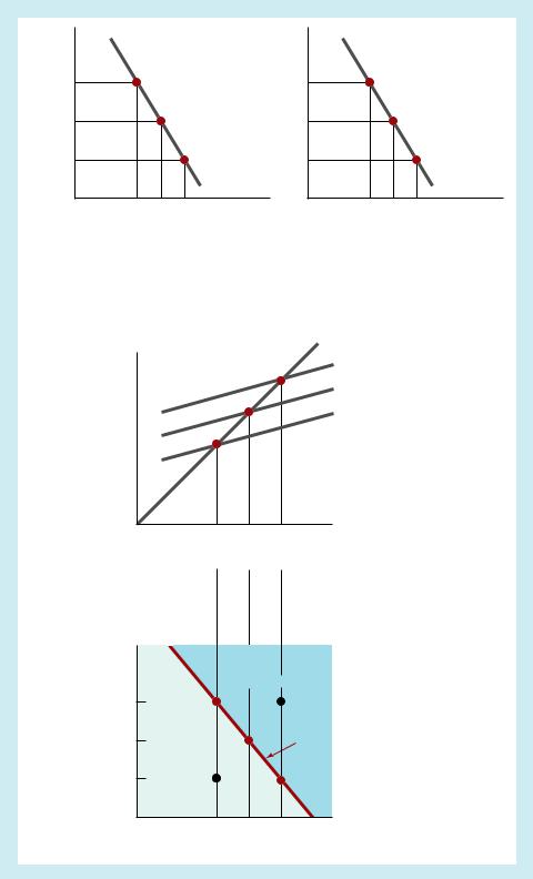
The relationship between the amount of planned investment spending and any given level of the interest rate is illustrated by the investment schedule in panel (a) of Figure 7. The downward slope of the schedule reflects the negative relationship between planned investment spending and the interest rate. At a low interest rate i1, the level of planned investment spending I1 is high; for a high interest rate i3, planned investment spending I3 is low.

Interest Rates and Net Exports. As discussed in more detail in Chapter 19, when interest rates rise in the United States (with the price level fixed), U.S. dollar bank deposits become more attractive relative to deposits denominated in foreign currencies, thereby causing a rise in the value of dollar deposits relative to other currency deposits; that is, a rise in the exchange rate. The higher value of the dollar resulting from the rise in interest rates makes domestic goods more expensive than foreign goods, thereby causing a fall in net exports. The resulting negative relationship between interest rates and net exports is shown in panel (b) of Figure 7. At a low

6More modern Keynesian approaches suggest that consumer expenditure, particularly for consumer durables (cars, furniture, appliances), is influenced by the interest rate. This interest sensitivity of consumer expenditure can be allowed for in the model here by defining planned investment spending more generally to include the interest-sensitive component of consumer expenditure.

F I G U R E 7 Deriving the IS Curve

The investment schedule in panel

(a) shows that as the interest rate rises from i1 to i2 to i3, planned investment spending falls from I1 to I2 to I3, and panel (b) shows that net exports also fall from N X1 to N X2 to N X3 as the interest rate rises. Panel (c) then indicates the levels of equilibrium output Y1, Y2, and Y3 that correspond to those three levels of planned investment and net exports. Finally, panel (d) plots the level of equilibrium output corresponding to each of the three interest rates; the line that connects these points is the IS curve.

C H A P T E R 2 3 The Keynesian Framework and the ISLM Model 553

Interest

Rate, i

i 3 3

i 2 2

i 1 1

Interest

Rate, i

i 3

i 2

i 1

Investment

Schedule

3

2

1

Net Exports

Schedule

I 3 I 2 I 1

NX3 NX2 NX1

Planned Investment Spending, I

Net Exports, NX

(a) Interest rates and planned

(b) Interest rates and net exports

investment spending


Aggregate Demand, Y ad


1


2


3


45°


Y3

Y2

Y1

Y = Y ad


Y ad = C + I

1

+ G + NX

1

1


Y ad = C + I

2

+ G + NX

2

2


Y ad = C + I

3

+ G + NX

3

3


(c) Keynesian cross diagram

Aggregate Output, Y

Interest


Excess


Rate, i


Supply


of Goods

i 3

3


B


i 2

Excess

2

IS

Demand


curve


for Goods


i 1

A

1


(d) IS curve


Y3

Y2

Y1

Aggregate Output, Y

554 P A R T V I Monetary Theory

interest rate i1, the exchange rate is low and net exports N X1 are high; at a high interest rate i3, the exchange rate is high and net exports N X3 are low.

Deriving the IS Curve. We can now use what we have learned about the relationship of interest rates to planned investment spending and net exports in panels (a) and (b) to examine the relationship between interest rates and the equilibrium level of aggregate output (holding government spending and autonomous consumer expenditure constant). The three levels of planned investment spending and net exports in panels

(a) and (b) are represented in the three aggregate demand functions in the Keynesian cross diagram of panel (c). The lowest interest rate i1 has the highest level of both planned investment spending I1 and net exports NX1, and hence the highest aggregate demand function Y ad1 . Point 1 in panel (d) shows the resulting equilibrium level of output Y1, which corresponds to interest rate i1. As the interest rate rises to i2, both planned investment spending and net exports fall, to I2 and NX2, so equilibrium output falls to Y2. Point 2 in panel (d) shows the lower level of output Y2, which corresponds to interest rate i2. Finally, the highest interest rate i3 leads to the lowest level of planned investment spending and net exports, and hence the lowest level of equilibrium output, which is plotted as point 3.

The line connecting the three points in panel (d), the IS curve, shows the combinations of interest rates and equilibrium aggregate output for which aggregate output produced equals aggregate demand.7 The negative slope indicates that higher interest rates result in lower planned investment spending and net exports, and hence lower equilibrium output.

What the IS Curve Tells Us. The IS curve traces out the points at which the total quantity of goods produced equals the total quantity of goods demanded. It describes points at which the goods market is in equilibrium. For each given level of the interest rate, the IS curve tells us what aggregate output must be for the goods market to be in equilibrium. As the interest rate rises, planned investment spending and net exports fall, which in turn lowers aggregate demand; aggregate output must be lower in order for it to equal aggregate demand and satisfy goods market equilibrium.

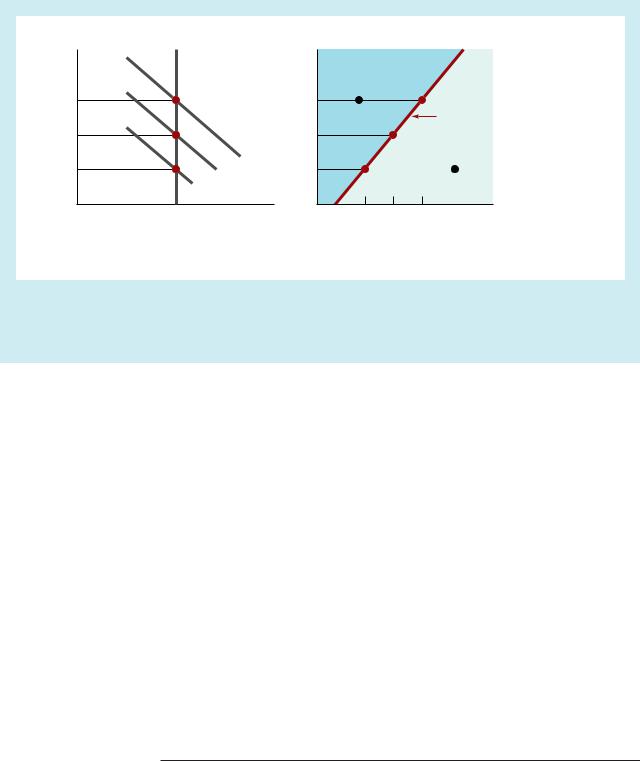
The IS curve is a useful concept because output tends to move toward points on the curve that satisfy goods market equilibrium. If the economy is located in the area to the right of the IS curve, it has an excess supply of goods. At point B, for example, aggregate output Y1 is greater than the equilibrium level of output Y3 on the IS curve. This excess supply of goods results in unplanned inventory accumulation, which causes output to fall toward the IS curve. The decline stops only when output is again at its equilibrium level on the IS curve.

If the economy is located in the area to the left of the IS curve, it has an excess demand for goods. At point A, aggregate output Y3 is below the equilibrium level of output Y1 on the IS curve. The excess demand for goods results in an unplanned decrease in inventory, which causes output to rise toward the IS curve, stopping only when aggregate output is again at its equilibrium level on the IS curve.

Significantly, equilibrium in the goods market does not produce a unique equilibrium level of aggregate output. Although we now know where aggregate output will head for a given level of the interest rate, we cannot determine aggregate output

7The IS was so named by Sir John Hicks because in the simplest Keynesian framework with no government sector, equilibrium in the Keynesian cross diagram occurs when investment spending I equals savings S.


C H A P T E R 2 3 The Keynesian Framework and the ISLM Model 555


because we do not know what the interest rate is. To complete our analysis of aggre-


gate output determination, we need to introduce another market that produces an


additional relationship that links aggregate output and interest rates. The market for


money fulfills this function with the L M curve. When the L M curve is combined with


the IS curve, a unique equilibrium that determines both aggregate output and the


interest rate is obtained.


Equilibrium in

Just as the IS curve is derived from the equilibrium condition in the goods market

the Market

(aggregate output equals aggregate demand), the L M curve is derived from the equi-

for Money: The

librium condition in the market for money, which requires that the quantity of money

LM Curve

demanded equal the quantity of money supplied. The main building block in KeynesÕs


analysis of the market for money is the demand for money he called liquidity prefer-


ence. Let us briefly review his theory of the demand for money (discussed at length in


Chapters 5 and 22).


KeynesÕs liquidity preference theory states that the demand for money in real


terms M d/P depends on income Y (aggregate output) and interest rates i. The demand


for money is positively related to income for two reasons. First, a rise in income raises


the level of transactions in the economy, which in turn raises the demand for money


because it is used to carry out these transactions. Second, a rise in income increases


the demand for money because it increases the wealth of individuals who want to


hold more assets, one of which is money. The opportunity cost of holding money is


the interest sacrificed by not holding other assets (such as bonds) instead. As interest


rates rise, the opportunity cost of holding money rises, and the demand for money


falls. According to the liquidity preference theory, the demand for money is positively


related to aggregate output and negatively related to interest rates.


Deriving the LM Curve. In KeynesÕs analysis, the level of interest rates is determined


by equilibrium in the market for money, at which point the quantity of money


demanded equals the quantity of money supplied. Figure 8 depicts what happens to


equilibrium in the market for money as the level of output changes. Because the L M


curve is derived holding the money supply at a fixed level, it is fixed at the level of M


in panel (a).8 Each level of aggregate output has its own money demand curve because


as aggregate output changes, the level of transactions in the economy changes, which


in turn changes the demand for money.


When aggregate output is Y , the money demand curve is M d (Y

1

) : It slopes


1


downward because a lower interest rate means that the opportunity cost of holding money is lower, so the quantity of money demanded is higher. Equilibrium in the market for money occurs at point 1, at which the interest rate is i1. When aggregate output is at the higher level Y2 , the money demand curve shifts rightward to M d (Y2 ) because the higher level of output means that at any given interest rate, the quantity of money demanded is higher. Equilibrium in the market for money now occurs at point 2, at which the interest rate is at the higher level of i2 . Similarly, a still higher level of aggregate output Y3 results in an even higher level of the equilibrium interest rate i3 .

8As pointed out in earlier chapters on the money supply process, the money supply is positively related to interest rates, and so the M s curve in panel (a) should actually have a positive slope. The M s curve is assumed to be vertical in panel (a) in order to simplify the graph, but allowing for a positive slope leads to identical results.

556 P A R T V I Monetary Theory


M s


Interest


Interest

Excess Supply of Money


Rate, i


Rate, i


i 3

3


i 3

A


3


2


LM Curve

i 2


i 2


2


M d(Y3)


i 1

1


Excess

B

M

d

(Y2)

i 1

1

Demand


M d(Y

)


for Money


1


_


M /P


Y1

Y2

Y3


Quantity of Real Money Balances, M/P

Aggregate Output Y

(a) Market for money

(b) LM curve

F I G U R E 8 Deriving the LM Curve


Panel (a) shows the equilibrium levels of the interest rate in the market for money that arise when aggregate output is at Y1, Y2, and Y3. Panel

(b) plots the three levels of the equilibrium interest rate i1, i2, and i3 corresponding to these three levels of output; the line that connects these points is the LM curve.

Panel (b) plots the equilibrium interest rates that correspond to the different output levels, with points 1, 2, and 3 corresponding to the equilibrium points 1, 2, and 3 in panel (a). The line connecting these points is the L M curve, which shows the combinations of interest rates and output for which the market for money is in equilibrium.9 The positive slope arises because higher output raises the demand for money and thus raises the equilibrium interest rate.

What the LM Curve Tells Us. The L M curve traces out the points that satisfy the equilibrium condition that the quantity of money demanded equals the quantity of money supplied. For each given level of aggregate output, the L M curve tells us what the interest rate must be for there to be equilibrium in the market for money. As aggregate output rises, the demand for money increases and the interest rate rises, so that money demanded equals money supplied and the market for money is in equilibrium.

Just as the economy tends to move toward the equilibrium points represented by the IS curve, it also moves toward the equilibrium points on the L M curve. If the economy is located in the area to the left of the L M curve, there is an excess supply of money. At point A, for example, the interest rate is i3 and aggregate output is Y1 . The interest rate is above the equilibrium level, and people are holding more money than they want to. To eliminate their excess money balances, they will purchase bonds, which causes the price of the bonds to rise and their interest rate to fall. (The inverse relationship between the price of a bond and its interest rate is discussed in

9Hicks named this the LM curve to indicate that it represents the combinations of interest rates and output for which money demand, which Keynes denoted as L to represent liquidity preference, equals money supply M.

C H A P T E R 2 3 The Keynesian Framework and the ISLM Model 557

Chapter 4.) As long as an excess supply of money exists, the interest rate will fall until it comes to rest on the L M curve.

If the economy is located in the area to the right of the L M curve, there is an excess demand for money. At point B, for example, the interest rate i1 is below the equilibrium level, and people want to hold more money than they currently do. To acquire this money, they will sell bonds and drive down bond prices, and the interest rate will rise. This process will stop only when the interest rate rises to an equilibrium point on the L M curve.

ISLM Approach to Aggregate Output and Interest Rates

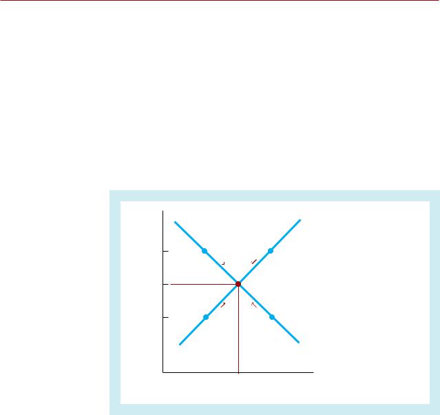
Now that we have derived the IS and L M curves, we can put them into the same diagram (Figure 9) to produce a model that enables us to determine both aggregate output and the interest rate. The only point at which the goods market and the market for money are in simultaneous equilibrium is at the intersection of the IS and L M curves, point E. At this point, aggregate output equals aggregate demand (IS ) and the quantity of money demanded equals the quantity of money supplied (L M ) . At any other point in the diagram, at least one of these equilibrium conditions is not satisfied, and market forces move the economy toward the general equilibrium, point E.

To learn how this works, letÕs consider what happens if the economy is at point A, which is on the IS curve but not the L M curve. Even though at point A the goods market is in equilibrium, so that aggregate output equals aggregate demand, the interest rate is above its equilibrium level, so the demand for money is less than the supply. Because people have more money than they want to hold, they will try to get rid of it by buying bonds. The resulting rise in bond prices causes a fall in interest rates,

F I G U R E 9 ISLM Diagram:

Simultaneous Determination of Output

and the Interest Rate

Only at point E, when the interest rate is i * and output is Y *, is there equilibrium simultaneously in both the goods market (as measured by the IS curve) and the market for money (as measured by the LM curve). At other points, such as A, B, C, or D, one of the two markets is not in equilibrium, and there will be a tendency to head toward the equilibrium, point E.

Interest

LM

Rate, i


A

B

i *

E

D

C


IS


Y *

Aggregate Output, Y

558 P A R T V I

Monetary Theory


which in turn causes both planned investment spending and net exports to rise, and


thus aggregate output rises. The economy then moves down along the IS curve, and


the process continues until the interest rate falls to i* and aggregate output rises to


Y *Ñthat is, until the economy is at equilibrium point E.


If the economy is on the L M curve but off the IS curve at point B, it will also head


toward the equilibrium at point E. At point B, even though money demand equals


money supply, output is higher than the equilibrium level and exceeds aggregate


demand. Firms are unable to sell all their output, and unplanned inventory accumu-


lates, prompting them to cut production and lower output. The decline in output


means that the demand for money will fall, lowering interest rates. The economy then


moves down along the L M curve until it reaches equilibrium point E.


Study Guide

To test your understanding of why the economy heads toward equilibrium point E at


the intersection of the IS and LM curves, see if you can provide the reasoning behind


the movement to point E from points such as C and D in the figure.


We have finally developed a model, the ISLM model, that tells us how both inter-


est rates and aggregate output are determined when the price level is fixed. Although


we have demonstrated that the economy will head toward an aggregate output level


of Y *, there is no reason to assume that at this level of aggregate output the economy


is at full employment. If the unemployment rate is too high, government policymak-


ers might want to increase aggregate output to reduce it. The ISLM apparatus indi-


cates that they can do this by manipulating monetary and fiscal policy. We will


conduct an ISLM analysis of how monetary and fiscal policy can affect economic


activity in the next chapter.


Summary

1.In the simple Keynesian framework in which the price level is fixed, output is determined by the equilibrium condition in the goods market that aggregate output equals aggregate demand. Aggregate demand equals the sum of consumer expenditure, planned investment spending, government spending, and net exports. Consumer expenditure is described by the consumption function, which indicates that consumer expenditure will rise as disposable income increases. KeynesÕs analysis shows that aggregate output is positively related to autonomous consumer expenditure, planned investment spending, government spending, and net exports and negatively related to the level of taxes. A change in any of these factors leads, through the expenditure multiplier, to a multiple change in aggregate output.

2.The ISL M model determines aggregate output and the interest rate for a fixed price level using the IS and L M

curves. The IS curve traces out the combinations of the interest rate and aggregate output for which the goods market is in equilibrium, and the LM curve traces out the combinations for which the market for money is in equilibrium. The IS curve slopes downward, because higher interest rates lower planned investment spending and net exports and so lower equilibrium output. The LM curve slopes upward, because higher aggregate output raises the demand for money and so raises the equilibrium interest rate.

3.The simultaneous determination of output and interest rates occurs at the intersection of the IS and LM curves, where both the goods market and the market for money are in equilibrium. At any other level of interest rates and output, at least one of the markets will be out of equilibrium, and forces will move the economy toward the general equilibrium point at the intersection of the IS and LM curves.

C H A P T E R 2 3 The Keynesian Framework and the ISLM Model 559

Key Terms

aggregate demand, p. 537

consumption function, p. 538

IS curve, p. 551

aggregate demand function, p. 541

disposable income, p. 538

LM curve, p. 551

Òanimal spirits,Ó p. 544

expenditure multiplier, p. 543

marginal propensity to consume,

autonomous consumer expenditure,

fixed investment, p. 539

p. 538


p. 538

government spending, p. 537

net exports, p. 537


consumer expenditure, p. 536

inventory investment, p. 539

planned investment spending, p. 536


QUIZ Questions and Problems

Questions marked with an asterisk are answered at the end of the book in an appendix, ÒAnswers to Selected Questions and Problems.Ó

1.Calculate the value of the consumption function at each level of disposable income in Table 1 if a 100 and mpc 0.9.

*2. Why do companies cut production when they find that their unplanned inventory investment is greater than zero? If they didnÕt cut production, what effect would this have on their profits? Why?

3.Plot the consumption function C 100 0.75Y on graph paper.

a.Assuming no government sector, if planned investment spending is 200, what is the equilibrium level of aggregate output? Show this equilibrium level on the graph you have drawn.

b.If businesses become more pessimistic about the profitability of investment and planned investment spending falls by 100, what happens to the equilibrium level of output?

*4. If the consumption function is C 100 0.8Y and planned investment spending is 200, what is the equilibrium level of output? If planned investment falls by 100, how much does the equilibrium level of output fall?

5.Why are the multipliers in Problems 3 and 4 different? Explain intuitively why one is higher than the other.

*6. If firms suddenly become more optimistic about the profitability of investment and planned investment spending rises by $100 billion, while consumers become more pessimistic and autonomous consumer

spending falls by $100 billion, what happens to aggregate output?

7.ÒA rise in planned investment spending by $100 billion at the same time that autonomous consumer expenditure falls by $50 billion has the same effect on aggregate output as a rise in autonomous consumer expenditure alone by $50 billion.Ó Is this statement true, false, or uncertain? Explain your answer.

*8. If the consumption function is C 100 0.75Y, I 200, and government spending is 200, what will be the equilibrium level of output? Demonstrate your answer with a Keynesian cross diagram. What happens to aggregate output if government spending rises by 100?

9.If the marginal propensity to consume is 0.5, how much would government spending have to rise in order to raise output by $1,000 billion?

*10. Suppose that government policymakers decide that they will change taxes to raise aggregate output by $400 billion, and mpc 0.5. By how much will taxes have to be changed?

11.What happens to aggregate output if both taxes and government spending are lowered by $300 billion and mpc 0.5? Explain your answer.

*12. Will aggregate output rise or fall if an increase in autonomous consumer expenditure is matched by an equal increase in taxes?

13.If a change in the interest rate has no effect on planned investment spending, trace out what happens to the equilibrium level of aggregate output as interest rates fall. What does this imply about the slope of the IS curve?

560 P A R T V I Monetary Theory

*14. Using a supply and demand diagram for the market for money, show what happens to the equilibrium level of the interest rate as aggregate output falls. What does this imply about the slope of the L M curve?

15.ÒIf the point describing the combination of the interest rate and aggregate output is not on either the IS or the L M curve, the economy will have no tendency to head toward the intersection of the two curves.Ó Is this statement true, false, or uncertain? Explain your answer.

Web Exercises

1.The study tip on page 538 suggests that you construct a consumption function based on your own propensity to consume. This process can be automated by using the tools available at http://nova.umuc.edu/~black /consf1000.html. Assume your level of consumer expenditure as $2,000 (input as 20) and that your marginal propensity to spend is 0.8. Review the resulting graphs. At an income level of $5,000 (50 on the graph), what is your expenditure?

2.Refer to question 1. Again go to http://nova.umuc

.edu/~black/consf1000.html. Input any level of consumer expenditure and marginal propensity to consume. According to the resulting graph, where do the 45¡ line and the consumption function cross? What is the significance of this point? Will you be a saver or dissaver at income levels below this point?

Соседние файлы в предмете [НЕСОРТИРОВАННОЕ]