Учебники / 0841558_16EA1_federico_milano_power_system_modelling_and_scripting

Fig. 1.1 UCTE interconnected system

provided by basic undergraduate courses on electrical machines and power systems. Moreover, several excellent books in the literature provide the fundamentals of power system operation, analysis, control and stability. Traditional references are [10, 52, 114, 160, 163, 179, 269, 294, 330, 355]. References that cover advanced topics while maintaining a comprehensive approach are [110, 147, 184, 263].

1.2Motivations

As a student, I su ered the deep hiatus between the aforementioned references, which provide theoretical tools, and the commercial computer-based implementations of power system models, which are almost impenetrable black boxes. There is often a huge gap between the equations typeset on a book page and the code that represents those equations in a form suitable for a computer. Unfortunately, it is not easy to find books that tries to cover this gap. This is quite surprising since nowadays no one is really doing any calculation by hand, at least for power system analysis. Thus, given that a book like Venikov’s “Transient Processes in Electrical Power Systems” is an evidence of what a pencil and a long Russian winter can inspire to a brilliant mind [330], it is time to systematically provide side by side to mathematical models the implementation of such models in some adequate computer language. Some examples of books that have attempted to follow such approach are [291] and [227] and, more recently [14], [17] and [2].

As a professor, I su er, even more than when I was a student myself, when observing students accepting acritically the results provided by some

software package. The idea that a computer only executes code and that the code has been written by some error-prone human being is too often beyond students’ imagination. Students also very often ignore the old programmer saying garbage in, garbage out, which means that if the input data (provided by the student) are inconsistent, the computer cannot do the miracle and return correct results.

Although based on the well established background of the references cited in Section 1.1, the purpose of this book is not to concentrate on some specific detail of power systems. Rather, the main goal is to provide, through a variety of examples, very general tools for approaching a systematic study of power systems. These tools are both methodological (modelling), structural (architecture) and practical (scripting). The ultimate object is to help the reader develop the ability of approaching power system analysis in a both critical and constructive way. This chapter is dedicated to modelling issues, while architecture and scripting matters are tackled in Chapters 2 and 3, respectively.

1.3Modelling Physical Systems

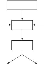
In the very first class of electrical circuits that I attended at the University of Genoa, the professor drew on the blackboard a scheme similar to the one depicted in Figure 1.2. The scheme shows the logical steps that an engineer has to follow to study a physical system. The first step is to define the model, which requires hypotheses and simplifications. Then, one has to formalize the model into equations. Finally, the equations have to be solved either in a closed form or numerically.

In this book, the “physical system” is a power system. In the past, analogical Transient Network Analyzers (TNAs) were the only simulation tools available for research and education in power engineering [10]. However, the advent of digital analysis has led to a more convenient way of performing simulations through digital computers [156]. Thus, in the book, it is assumed that the model is a simplified representation of the physical system suitable for being expressed in terms of mathematical equations and translated into computer programing code.

The scheme of Figure 1.2 is actually an old concept by Plato. In the “Sophist”, Plato defines the science (e.g., the real knowledge) as (e.g., an imitation technique based on the experience). Thus, the engineer that formulates mathematical models corresponds to the philosopher. Actually, one of the goals of this book is to show that modelling does not consist simply in writing a set of equations but implies a “philosophical” view of physical phenomena.

A delicate point that has to be emphasized is that both simplifications and hypotheses are often driven by the numerical solution methods that are available for solving the given system equations. Even more critical is the importance of simplifications if one looks for an analytical explicit solution. Indeed, it is a pity that students do not solve anything by hand anymore.

Physical system

Model

Equations

Fig. 1.2 General approach for studying a physical system

Good ideas often comes out just to avoid a repetitive work. In this regard, a computer programming saying states that very good programmers are often very lazy men.

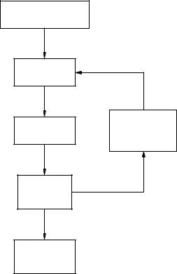
In conclusion, the simple feed-forward scheme shown in Figure 1.2 has to be modified as in Figure 1.3. For the sake of realism, the analytical solution block has been removed from Figure 1.3. The key point of Figure 1.3 is that between the equations and the numerical solution blocks there is a key step, namely the translation of the equations in a suitable code using available algorithms. As any translation, programming is not a trivial step and cannot be neglected.

Example 1.1 Optimal Placement of Capacitor Banks

In order to describe with a qualitative example the modelling issues discussed above, consider the problem of finding the optimal bus positions of a given number nc of capacitor banks that minimizes power system losses. The positions of the capacitor banks can be conveniently described by a vector u of order nb of binary variables, where nb is the number of system buses. The Boolean variable associated to each bus is 1 if the bank is installed at that bus, 0 otherwise. Since system losses are defined by the set of power flow equations that are intrinsically nonlinear, the resulting optimization problem belongs to the class of mixed integer nonlinear programming (MINLP) problems.

Physical system

Model

Simplifications

Available algorithms

Numerical

solution

Fig. 1.3 Modified general approach for studying a physical system

This MINLP problem can certainly be solved, it is just a matter of time. In fact, an evident solution is to try all possible permutations nb!/(nb − nc)! of the vector u. Unfortunately, even for small values of nb and nc, the number of permutations is huge and the required simulation time of trying all permutations is intractable. Actually, MINLP problems cannot be solved using a well-assessed and commonly accepted algorithm similar to, for example, the LU factorization. Thus, formulating the problem as a MINLP does not conclude the modelling phase. Further modelling e ort is needed to make the problem solvable.

A common strategy is to adopt adequate simplifications or decomposition techniques to transform a MINLP either in a mixed integer linear programming (MILP) problem, thus eliminating nonlinearity, or in a nonlinear programming (NLP), thus eliminating integer variables.

In order to describe the need of the feedback included in Figure 1.3, assume, only for the sake of example, that u can be modelled as a vector of continuous variables through the following constraint:

Equation (1.1) may lead to think that the original MINLP problem can be promptly converted into a nonlinear programming (NLP) one. Unfortunately equation (1.1) is a highly nonlinear constraint that generally leads to so severe convexity issues that it is practically impossible to find the global optimum. Thus this is an example of modelling inconsistency driven by a poor knowledge of NLP solvers.

Of course, in the literature, one can find a variety of methods for solving the proposed MINLP problem. In particular, it can be approached using a Benders’ decomposition [204]. Other techniques based on artificial intelligence can be e cacious as well [169]. All these techniques attempt to reduce as much and as “smartly” as possible the number of permutations to be taken into account.

The first conclusion is that there is generally no easy shortcut for avoiding the complexity due to a combinatorial problem. The second conclusion, which is more relevant for the scope of this book, is that without an adequate knowledge of algorithms and numerical methods, one may set up an inconsistent model. Since engineers are often interested more in the solution than in the model itself, an unsolvable model is useless.

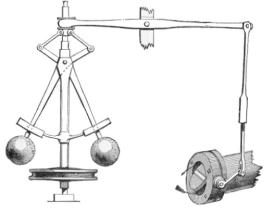
Example 1.2 Flyball Governor Model

As another qualitative example, consider the problem of the classical James Watt’s centrifugal control (see Figure 1.41). This control system allows controlling the speed of an engine by regulating the amount of fluid flow. The centrifugal control has been widely used for steam turbines of electric power generators for maintaining synchronism (e.g., flyball and isochronous governors). The main principle is as follows: a set of flyballs (or fly weights), which rotate driven by the engine to be controlled, is connected to levers whose position actuates on the steam valve (throttle). An increase in the engine speed results in a centrifugal force increase. The latter raises the weights and thereby reduces the steam flow into the engine. Finally, the steam flow decrease causes a reduction in the engine speed.

There is always a delay between the time at which the engine speed varies and the time at which the steam flow is reduced by the centrifugal control [182]. Actually, any steam turbine governor control intrinsically su ers of time delays. As a matter of fact, a thermal plant consists of several heat transfer apparatus connected together by pipes. An adequate modelling of transport delays introduced by these pipes is desirable to calculate system transient behavior. If the fluid velocity through the pipe is constant, the

1Picture obtained from Science Fair Project Encyclopedia, available at www.all- science-fair-projects.com

Fig. 1.4 Flyball governor

transfer function of the piping lag is also constant. However, if the velocity of the fluid is a function of time, the delays become time dependent.

An accurate modelling of variable time delays complicates considerably the analysis since it is not possible to define a standard transfer function of the system. As in Example 1.1, the main issue is the mathematical complexity inherent variable time delay (or retarded ) systems. These belong to the class of functional di erential equations (FDEs) that are infinite dimensional, as opposed to the finite dimension of ordinary di erential equations (ODEs). In order to explain the complexities that raises when studying retarded systems, it su ces to say that, for FDEs, there is an infinite number of trajectories that passes for a given state x(t). As a matter of fact, in FDEs, the state is a function of a past time-interval [t − τ (t), t], where τ > 0 is the time delay, which is possibly a function of time. Another di culty is that it is not possible to define a state matrix for FDEs as it is usual practice for ODEs. For this reason research is in progress to assess the e ects of time delays on system stability [258].

Regarding the steam turbine regulator, the common solution, that avoids time-delay issues, is to model the control as an ODE. As a matter of fact, time delays are often neglected and, along with other simplifications, the resulting di erential equations used for modelling turbine governors are linear [10]. Further discussion on turbine governors is given in Chapter 16.

Example 1.3 Inductor Model

Any basic circuit theory course introduces the concept of inductance, whose well-known constitutive di erential equation is

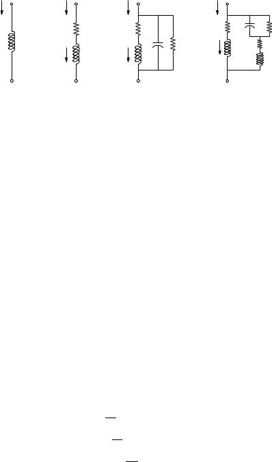
Fig. 1.5 Various detail degree models of a inductor winding: (a) ideal inductance;

(b) fundamental frequency model; (c) second-order model; and (d) third-order model. The schemes only show electrical quantities

where L is a constant parameter called inductance and di/dt is the first time derivative of the current flowing in the device (see Figure 1.5.a).

However, ideal inductances do not exist. In other words, there is no physical device whose terminal voltage can be exactly described by the di erential equation (1.2). The physical device whose behavior is close to an ideal inductance is the inductor. Inductors are made by a coil wound on an iron core. A winding is characterized by a resistance R, hence the model of a real device have to take into account Ohmic losses. Moreover, the magnetic properties of the iron are not ideal, hence the relation between the total magnetic flux φ and the electrical current i is not linear. A more realistic model of the inductive winding is as follows (see Figure 1.5.b):

This model can be adequate in case of constant temperature and low frequency. Otherwise, one has to take into account the dependence of the resistance R on the temperature Θ and the capacitive e ects among coils and between the coils an the ground. Such e ects can be modeled using introducing a lumped parasitic (or hearting) capacity C in parallel with the inductance (see Figure 1.5.c). One can also include a conductance G in parallel with the capacitance to take into account the skin resistance of the winding. The resulting model is as follows:

dφ

v = dt + R(Θ)iL(φ) (1.4)

dv

i = C dt + iL(φ) + Gv

Ri2L = mg cp dΘdt + kA(Θ − Θa)

where iL is the current circulating in the winding, i the total current that flows in the inductor, mg is the winding mass, cp is the equivalent specific heat of the winding, k the convective heat transfer coe cient, A the winding active area and Θa the ambient temperature. Both the electrical and the thermodynamical models can be further complicated. For example, Figure 1.5.d shows a third-order model of an inductor [168].

The most precise electrical model that can be formulated for the inductor is based on Maxwell’s and constitutive equations:

field, d is the electric flux density, j is the electric current density, is the

charge density, μ is the magnetic permeability, ς is the electric conductivity, and ε is the electric permittivity. Equations (1.5) have to be particularized with adequate boundary conditions and, in general, have to be solved numerically using, for example, a finite-element three-dimensional approach [82].

Even without entering into the mathematical details of modelling the inductor as a continuum, one can easily anticipate that the computational burden of modelling an entire power system using such approach as well as the amount of information that should be processed is intractable. Too much information can result in no information. Even though in the literature there are some proposals of modelling a power system as a continuum [274, 308], the continuum approach remains so far only an academic, though intriguing, exercise.

The main conclusion that can be drawn by this example is that the upper boundary to the details that can be taken into account in a mathematical model is driven by the computational limits of available computers and by the ability of processing and analyzing results. As it is discussed in Part II, in the past, such limits have led to some approximations that are nowadays considered standards de facto but that are not really binding anymore.

1.4Hybrid Dynamical Model

One should gather from the discussions and the examples provided in the previous sections that a power system consists of a set of devices that can be described by continuous dynamics as well as discrete events. Synchronous machines can be adequately modelled using a set of nonlinear ordinary di erential equations (ODEs) as long as lumped parameters are used. Most controllers can also be modelled using ODEs as long as time-dependent delays are approximated with lags or simply neglected. Discrete events or, which is the same, discrete variables are also an essential part of power systems.

For example, the tap position of voltage regulating transformers and breaker statuses are discrete variables.

If one assumes that the status of discrete variables is known or can be reasonably guessed, then, for each discrete variable change, the system jumps from one set of continuous equations to another. In order to clarify this point, it su ces to think of the consequence of opening a breaker of a transmission line. Before opening the breaker the line is connected and the power flow through the line itself can be defined using well-known continuous equations. After opening the breaker, the line is disconnected and thus its equations have to be removed from the model.2 Except for the fact that before and after the breaker intervention, power flow equations are di erent, there is no need of modelling the status of the breaker as a discrete variable. Of course, a completely di erent issue would be to find the best transmission line arrangement that minimize a certain aspect of the power system, say, for example, losses. In this case the problem is again combinatorial and breaker statuses have to be used as Boolean variables. However, while simulating the power system behavior, the status of the lines (as well as of most devices) is known and one has not have to deal with a MINLP problem.

The most general model that can be used for representing power systems is as follows:

where ξ (ξ Rnξ ) is the vector of state variables, u (u Rnu ) the vector of discrete variables, t (t R+) the time, and ϕ (ϕ : Rnξ × Rnu × R+ → Rnξ ) the vector of di erential equations. As previously discussed, u have generally not to be determined but are fixed to a given value and then changed to enforce system transients. For example, opening a breaker can be required for clearing a fault and can be driven by an over-current protection. If one want to avoid using the vector u, (1.6) can be rewritten as follows:

≥

where ti is the breaker intervention time. Clearly, if more than one discrete variable changes value, the if-then rule is more complex. In conclusion, whenever is possible to transform a discrete variable u as an if-then condition, the discrete variable can be eliminated from the equation at the cost of splitting ϕ as in (1.7).

It has to be noted that, in (1.7), both ϕ− and ϕ+ are continuous and smooth (i.e., di erentiable) functions. This fact is important since one can use any numerical method for nonlinear equations (e.g., Newton’s method) and standard stability analysis (e.g., eigenvalue analysis) when studying (1.7).

2The case of under load tap changers is slightly more complex and is discussed in Subsection 11.2.2 of Chapter 11.

Equations (1.6) as well as (1.7) imply that any variable of the system is a state. This assumption is in agreement with the Leibniz’s axiom: natura non facit saltus (i.e., nature does not jump). This is certainly an excellent approximation for macroscopic dynamical systems. However, when dealing with power system analysis the time constants of di erent phenomena can span a wide time range. Figure 1.6 depicts the time scales of a variety of typical phenomena and controls that are of interest in power system analysis. Since the time scales span from micro-seconds to several hours, taking into account the dynamics of each phenomena in an unique model would results in an intractable system.

The common solution to this issue is to divide the vector of general state variables ξ into three sub-vectors: (i) state variables ξs characterized by slow dynamics (i.e., big time constants), (ii) state variables ξi whose dynamics are of interest, and (iii) state variables ξf characterized by fast dynamics (i.e., small time constants). In mathematical terms, one has:

where ξ = [ξTs , ξTi , ξTf ]T . In (1.8), the time evolution of ξs can be considered so slow that their variations can be neglected (e.g., ξs are frozen at a given value). On the other hand, the dynamics of ξf can be considered so fast that their variations can be considered instantaneous.

The consequences of the approximation described above are twofold: ξs are constant and can be considered controllable parameters; and the state variables ξf can be considered algebraic variables, i.e., variables whose variations are instantaneous. Thus, algebraic variables can facere saltus (i.e., jump) from one value to another and can be discontinuous.

The resulting model is thereby a set of nonlinear di erential algebraic equations (DAEs) with discrete variables, as follows:

where x (x Rnx ) indicates the vector state variables, y (y Rny ) are