

Учебники / 0841558_16EA1_federico_milano_power_system_modelling_and_scripting
.pdf96 |
4 Power Flow Analysis |
Example 4.5 Distributed Slack Bus Power Flow for the IEEE 14-Bus System
Table 4.5 shows the results of the power flow with distributed slack bus model for the IEEE 14-bus test system. The loss participation factors of generators 1 and 2 are γ1 = γ2 = 1. Furthermore, pG0,1 = 2.3 pu for the slack bus. In this case, the final generated powers are very similar to the single slack bus model. This result is a consequence of the fact that pG0,1 pG0,2.
Table 4.5 Power flow results for the IEEE 14-bus system with distributed slack bus model
Bus |
v |
θ |
pG |
qG |
pL |
qL |
h |
[pu] |
[rad] |
[pu] |
[pu] |
[pu] |
[pu] |
|
|
|
|
|
|
|
|
|
|
|
|
|
|
1 |
1.06 |
0 |
2.32 |
−0.1647 |
0 |
0 |
2 |
1.045 |
−0.0868 |
0.4035 |
0.4342 |
0.217 |
0.127 |
3 |
1.01 |
−0.2219 |
0 |
0.2507 |
0.942 |
0.19 |
4 |
1.018 |
−0.1799 |
0 |
0 |
0.478 |
−0.039 |
5 |
1.02 |
−0.153 |
0 |
0 |
0.076 |
0.016 |
6 |
1.07 |
−0.2481 |
0 |
0.1273 |
0.112 |
0.075 |
7 |
1.062 |
−0.233 |
0 |
0 |
0 |
0 |
8 |
1.09 |
−0.233 |
0 |
0.1762 |
0 |
0 |
9 |
1.056 |
−0.2606 |
0 |
0 |
0.295 |
−0.0459 |
10 |
1.051 |
−0.2634 |
0 |
0 |
0.09 |
0.058 |
11 |
1.057 |
−0.258 |
0 |
0 |
0.035 |
0.018 |
12 |
1.055 |
−0.263 |
0 |
0 |
0.061 |
0.016 |
13 |
1.05 |
−0.2644 |
0 |
0 |
0.135 |
0.058 |
14 |
1.036 |
−0.2797 |
0 |
0 |
0.149 |
0.05 |
|
|
|
|
|
|
|
Totals |
|
|
2.724 |
0.8237 |
2.59 |
0.5232 |
4.5A General Framework for Power Flow Solvers
Let us consider a set of autonomous ODE:
y˙ |
˜ |
(4.68) |
= f (y) |
The simplest method of numerical integrating (4.68) is the explicit Euler’s method, as follows:
y |
(i) |
˜ |
(i) |
) |
(4.69) |
|
= Δtf (y |
|
|||
y(i+1) |
= y(i) + |
y(i) |
|
||
where Δt is a given step length.
4.5 A General Framework for Power Flow Solvers |
97 |
The analogy between (4.40) and (4.69) is straightforward if one defines:
f˜(y) = −[gy ]−1g(y) |
(4.70) |
Equations (4.40) can thus be viewed as the ith step of the Euler’s forward method where Δt = 1 [127]. Furthermore, robust Newton’s methods (4.48) are nothing but the ith step of the Euler’s integration method where Δt = α. In other words, the computation of the optimal multiplier α corresponds to a variable step forward Euler’s method.
Equations (4.68) and (4.70) leads to:
y˙ = −[gy ]−1g(y) |
(4.71) |
which is known as continuous Newton’s method. |
|
The equilibrium point y0 of (4.71) is |
|
0 = f˜(y0) = −[gy |0]−1g(y0) |
(4.72) |
Thus, assuming that gy is not singular, y0 is also the solution of (4.8). Assuming a non-singular Jacobian matrix for the power flow equations is an implicit hypothesis of any power flow analysis based on the factorization of gy (see also the discussion in Section 5.4 of the Chapter 5).
4.5.1Stability of the Continuous Newton’s Method
Di erentiating (4.70) with respect to y leads to:
˜ |
T ˜ |
(4.73) |
f y = y f (y) |
||
=−[gy ]−1gy − ( Ty ([gy ]−1))g(y)
=−Iny − ( Ty ([gy ]−1))g(y)
where Iny is the identity matrix of order ny . Since the equilibrium point y0 is a solution for g(y0) = 0, one has:
˜ |
= −Iny |
(4.74) |
f y |0 |
To prove equation (4.74) let us define the following quantities, based on tensor notation:
˜ |
˜ |
fi |
element i of the vector function f (y). |
gk |
element k of the vector function g(y). |
aik |
element (i, k) of the matrix [gy ]−1. |
˜ |
˜ |
fi,j |
partial derivative of fi with respect to the variable yj . |
gk,j |
partial derivative of gk with respect to the variable yj . |
aik,j |
partial derivative of aik with respect to the variable yj . |

98 |
4 Power Flow Analysis |
˜
For simplicity, the dependence of fi,j , gk,j and aik,j on y is omitted. Equations (4.70) and (4.73) can be rewritten as follows:
˜ |
ny |
|
|
|
|
(4.75) |
|
fi = − |
aik · gk |
|
|
|
k=1 |
|
|
˜ |
ny |
ny |
|
|
|
(4.76) |
|
fi,j = − |
aik · gk,j − |
aik,j · gk |
|
|
k=1 |
k=1 |
|
Since the matrix [aik ] is the inverse of gy , then
ny |
1 |
if |
i = j |
|
|
|
|||
0 |
|
|
|
|
aik · gk,j = |
if |
i = j |
(4.77) |
|
k=1 |
|
|
|
|
Thus, (4.76) can be written in the compact form:
˜ |
n |
|
|
(4.78) |
|
fi,j = −δij − aik,j · gk |
||
k=1
where δij is the well-known Kronecker’s operator. Furthermore, if gk = 0 k = 1, . . . , ny (which is verified at the solution y0), then one obtains the final expression:
˜ |
(4.79) |
fi,j = −δij |
that is the tensor version of (4.74).
This result is straightforward for a scalar g(y), i.e. for y R and g R, as follows:
|
|
˜ |
|
|
g(y) |
||||
|
|
y˙ = f (y) = |
− |
|
|
|
|
||
|
|
gy(y) |
|||||||
|
˜ |
|
gy(y) |
|
|
|
gyy(y) |
||
|
fy (y) = − |
|
+ |
|
|
g(y) |
|||
gy(y) |
gy2(y) |
||||||||
= −1 + gyy (y) g(y) gy2(y)
(4.80)
(4.81)
˜ |
|
|
thus fy(y0) = −1 if g(y0) = 0 and gy(y0) = 0. |
˜ |
at the solution point |
Equation (4.74) implies that all eigenvalues of f y |
||
are equal to −1. Thus, (4.74) means that the solution of (4.8), if exists, is asymptotically stable. The reachability of this solution depends on the starting point y(t0) = y(0), which has to be within the region of attraction or stability region of the equilibrium point y0.
The continuous Newton’s method is expected to show better ability to converge than other methods previously discussed if the initial guess is within
4.5 A General Framework for Power Flow Solvers |
99 |
the region of attraction. A case study that confirms this hypothesis is given in [196].
Example 4.6 Runge-Kutta’s Formula for Solving the Power Flow Problem
It is well-known that the forward Euler’s method, even with variable time step, can be numerically unstable. Reference [127] suggests that, given the analogy between the power flow equations (4.8) and the ODE (4.68), any well-assessed numerical method can be used for integrating (4.68). It is thus intriguing to use some e cient integration method for solving (4.8). Since
˜ − −1
the computation of f = [gy ] g implies the inversion of the power flow Jacobian matrix, only explicit integration methods are suitable and computationally e cient, since one does not need to compute the Jacobian matrix
˜
of f . Explicit numerical integration methods, including a variety of RungeKutta’s formulæ are described in Subsection 8.3.1 of Chapter 8.
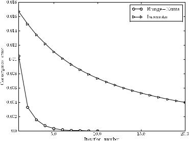
It is worth noting that any order and any version of explicit integration method can be used, and any of these methods is expected to be numerically more stable than the Euler’s forward method. For example, Figure 4.10 compares the convergence behavior of continuous Newton’s method solved using the classical 4th order Runge-Kutta’s formula (8.35) (see Example 8.2
Fig. 4.10 Convergence behavior of Runge-Kutta’s 4th order formula and the Iwamoto’s method for the IEEE 14-bus system
100 |
4 Power Flow Analysis |
of Chapter 8) and the Iwamoto’s method for the IEEE 14-bus system. The use of a robust power flow solver algorithm is not required in this case since this is a well-conditioned case. However, the results confirm that the RungeKutta’s formula converges faster than a variable step Euler’s method (e.g., Iwamoto’s method).
Script 4.6 Runge-Kutta’s Formula for Solving the Power Flow Problem
The Python implementation of the generic ith iteration of the Runge-Kutta’s 4th order formula (8.35) provided in Chapter 8 looks as follows:
yold = system.DAE.y
k1 = alfa*calcInc() system.DAE.y = yold + 0.5*k1
k2 = alfa*calcInc() system.DAE.y = yold + 0.5*k2
k3 = alfa*calcInc() system.DAE.y = yold + k3
k4 = alfa*calcInc() |
|
|
|
# compute RK4 increment of variables |
|
|
|
inc = (k1 + 2*(k2+k3) + k4)/6 |
|
|
|
# to estimate RK error, use the RK2:Dy and RK4:Dy. |
|
|
|
csi = max(abs(abs(k2) - abs(inc))) |
|
|
|
if csi > 0.01: |
|
|
|
deltat = max([0.985*deltat, |
0.75]) |
|
|
else: |
|
|
|
deltat = min([1.015*deltat, |
0.75]) |
|
|
system.DAE.y = yold + inc |
|
|
|
|
˜ |
(i) |
). The code above has to |
where it is assumed that calcInc() returns f (y |
|
||
be inserted in a while-loop similar to that discussed in Script 4.2. |
|||
4.6 Summary
This section summarizes most relevant concepts related to power flow analysis.
Power flow problem vs. classical circuit analysis: The power flow analysis di ers from classical circuit analysis in what concerns input data. Typical circuit input data are generator voltage phasors and load impedances. Thus, circuit analysis problem formulation is based on current injections that result in a linear problem if all parameters are constant. On the
4.6 Summary |
101 |
other hand, typical power flow data are load power consumptions and generator active power supplies. Thus, the power flow problem formulation is based on power injections that result in a nonlinear set of algebraic equations. The intrinsic nonlinearity of the power flow problem makes its solution a challenge.
System model: The classical power flow problem formulation considers only constant PV generators and constant PQ loads. Furthermore, one generator, the slack, is defined as slack and is used as phase angle reference. These models are deduced based on practical assumptions and operation of transmission systems. However, the classical power flow problem formulation can be improved in a variety of ways. For example, the distributed slack model is a better description of the behavior of the system than the standard single slack model. Other improvements of the classical models concerns the inclusion of detailed models of regulating transformers and dynamic devices. The entire Part III is devoted to provide further insights on detailed power flow models.
Power flow solvers: The classical formulation of the power flow problem can be solved only numerically. With this aim, several methods are available, including but not limited to: Gauss-Seidel’s, Jacobi’s, Newton’s, FDPF, and dc power flow methods. The Newton’s method is available in several versions: inexact (e.g., GMRES), dishonest and robust.
Dc power flow: The dc power flow formulation avoids the issues originated by the nonlinearity of the classical power flow problem. The dc formulation allows simplifying the equations so that only active power mismatches and bus voltage phase angles are considered. The resulting problem is linear but completely neglects reactive power flows and bus voltage magnitude deviations. For this reasons, the error introduced by the dc power flow model are not negligible.
General framework for power flow analysis solvers: Power flow algorithms based on the Newton’s method and its variants can be viewed as particular implementations of a general class of solvers, namely the continuous Newton’s method. This approach shows that the map of an iterative method is formally equivalent to find the equilibrium point of a set of differential equations. The equilibrium point of the equivalent ODE system is the solution of the power flow problem.
Chapter 5
Continuation Power Flow Analysis
This chapter describes a variety of techniques used for determining the point of collapse of power flow equations with particular emphasis on continuation power flow analysis. Section 5.1 introduces the maximum loading condition problem using a didactic 2-bus system. Section 5.2 defines the general model for the maximum loading condition. Section 5.3 describes direct methods for computing saddle-node bifurcation and limit-induced bifurcation points while Section 5.4 describes the continuation power flow technique. Section 5.4 also explains the conceptual di erences, advantages and drawbacks of continuation (or homotopy) methods with respect to direct ones. Subsections 5.4.4 and 5.4.5 discuss the analogy between the continuous Newton’s method and the homotopy approach and the N −1 contingency analysis, respectively. Finally, Section 5.5 summarizes the main concepts of the continuation power flow analysis.
5.1Background
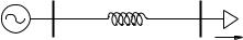
A relevant problem of power system analysis is the determination of the maximum load power consumption that a network can supply. With this aim, consider the 2-bus test system depicted in Figure 5.1. A similar example considering voltage dependent load characteristics can be found in Example 14.1 of Chapter 14.
1 |
2 |
|
jxL |
v1 + j0 |
p2 + jq2 |
Fig. 5.1 2-bus system
F. Milano: Power System Modelling and Scripting, Power Systems, pp. 103–130. springerlink.com c Springer-Verlag Berlin Heidelberg 2010

104 |
5 Continuation Power Flow Analysis |
The power flow equations that describe this system are:
|
|
v vref |
|
|
|
|
− p2 |
= |
2 |
1 |
|
sin θ2 |
|
xL |
|
|
||||
|
= |
v2 |
|
|
v2vref |
cos θ2 |
−q2 |
2 |
− |
1 |
|||
xL |
|
xL |
||||
where we assume that the slack generator voltage at bus 1 is reference. After some simple manipulations, one obtains:
|
|
|
|
2 |
|
v22 |
(v1ref )2 |
2 |
|
|
|
|
|
||||
|
|
|
|
p2 |
= |
|
|
|
sin |
θ2 |
|
|
|
||||
|
|
|
|
|
2 |
|
|
|
|
||||||||
|
|
|
|
|
|
|
|
x |
|
|
|
|
|
|
|
|
|
|
|
|
|
|
|
|
|
L |
|
|
|
|
|
|
|
|
|
2 |
|
v4 |
|
v2 |
|
v2 |
(vref )2 |
2 |
|
|
|
|
|
||||
|
2 |
|
2 |
|
|
2 |
1 |
|
|
|
|
|
|
||||
q2 |
+ |
|
+ 2q2 |
|
|
= |
|
|
|
cos θ2 |
|
|
|
||||
2 |
xL |
|
2 |
|
|
|
|
||||||||||
|
|
x |
|
|
|
x |
|
|
|
|
|
|
|
|
|
||
|
|
L |
|
|
|
|
|
L |
|
|
|
|
|
|
|
|
|
|
|
|
|
|
|
|
2 |
2 |
|
|
v4 |
|
v2 |
|
v2 |
(vref )2 |
|
|
|
|
|
|
|
|
|
2 |
|
2 |
|
2 |
1 |
||||
|
|
|
|
0 = p2 |
+ q2 |
+ |
|
|
+ 2q2 |
|
− |
|
|
||||
|
|
|
xL2 |
xL |
|
xL2 |
|||||||||||
(5.1)
the phase
(5.2)
The load bus voltage magnitude v2 can be written as a function of the load power p2:
v2 = −(q2xL − (v1ref )2/2) ± (q2xL − (v1ref )2/2)2 − x2L(p22 + q22) (5.3)
Assuming, without loss of generality, that the load has a constant power factor, i.e., q2 = p2 tan φ2, (5.3) becomes:
v2 = |
|
|
|
|||
−a ± |
a2 − xL2 p22(1 + tan2 φ2) |
(5.4) |
||||
where: |
(vref )2 |
|
||||
a = p2 tan φ2xL − |
(5.5) |
|||||
1 |
|
|||||
2 |
|
|||||
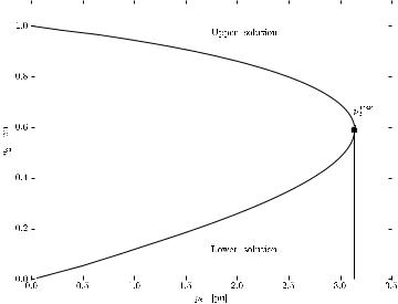
Equation (5.4) is depicted in Figure 5.2 and is known as PV curve or nose curve, due to its characteristic shape. It may be of interest to note that, in order to plot the PV curve of Figure 5.2, using (5.4) is not the best choice because the function v2(p2) is not defined on all R and is not biunivocal. To use the other way round, i.e., the function p2(v2) results easier:
p2 = v22 |
− |
|
|
|
|
|
|
|
(5.6) |
||
|
2 |
− − |
v2 |
|
|||||||
|
|
|
|
tan φ2 + |
|
tan2 φ2 |
1 |
(vref )2 |
|
|
|
|
|
|
|
|
1 |
|
|
|
|||
|
|
|
|
2 |
|
|
|
||||
|
xL |
|
1 + tan |
φ2 |
|
|
|
||||
|
|
|
|
|
|
|
|
|
|
|
|
|
|
|
|
|
|
|
|
|
|
|
|
5.1 Background |
105 |
|
|
|
|
|
|
|
Fig. 5.2 PV curve for the 2-bus system
Some relevant remarks on (5.4) are:
1.The system is characterized by a maximum value of the load power, say pmax2 , which is known as maximum loading condition.
2.For p2 > pmax2 the power flow equations (5.1) have no solution. For this reason, the power flow solution for p2 = pmax2 is known as point of collapse. In physical terms, this means that the system cannot supply a load whose power is p2 > pmax2 . Thus, pmax2 is the maximum power that can be transmitted by the network and it can be considered a limit of the transmission system.
3.For p2 < pmax2 , there are two values of v2 that solve (5.1). However, only the solution with the higher v2 value (upper solution) is physically acceptable. The other value (lower solution) has only a mathematical interest.
4.The shape of the PV curve is independent of the load power factor, as well as of system parameters. In other words, any network of any size and complexity shows a similar relationship between bus voltage magnitudes and load powers. PV curves are inherent the structure of classical power flow equations. As a matter of fact, as shown in (4.16) or (4.18), these have a quadratic dependence on bus voltages.
The PV curve depicted in Figure 5.2 was obtained assuming that the slack generator at bus 1 can supply any amount of active and reactive power. If the hypothesis about the reactive power is removed, there can be a value of

106 |
5 Continuation Power Flow Analysis |
p2 for which the reactive power generated by the slack bus is the maximum one, say q1max. Since the system has no other reactive power source, the load power cannot be increased any further. If the generator reactive power limit is reached before the transmission system limit, the former yields the point of collapse or, which is the same, the pmax2 value.
In order to determine the collapse point due to reactive power limit for the 2-bus system, assume that the slack is modelled as a constant QV generator, where q1 = q1max. The resulting power flow equations are:
− p2 |
= |
v2v1 |
sin θ2 |
(5.7) |
|||
xL |
|
||||||
|
= |
v2 |
|
|
v2v1 |
cos θ2 |
|
−q2 |
2 |
|
− |
|
|||
xL |
xL |
||||||
max |
= |
v2 |
|
|
v2v1 |
cos(−θ2) |
|
1 |
|
− |
|
||||
q1 |
|
|
|
||||
xL |
xL |
||||||
In this case, the voltage magnitude v1 is a variable. Using the second and the third equations of (5.7), one has:
v1 = xLq1max + v22 + xLp2 tan φ2 (5.8)
Then, substituting (5.8) in (5.2), the expression of p2(v2) becomes:
p2 = |
xL tan φ2 |
+ |
|
( xL |
2 |
+ |
2 |
2 1 |
2 L |
(5.9) |
|||
|
|
v22 |
|
|
|
|
v22 |
tan φ )2 |
|
4v2qmax(1 + tan2 |
φ )/x |
|
|
|
|
|
|
|
|
|
|||||||
|
|
|
|
|
|
|
|
2(1 + tan |
|
φ2) |
|
|
|
If (5.6) and (5.9) intersect in the upper part of (5.6), then the generator reactive power limit occurs before the transmission system limit. This situation is illustrated in Figure 5.3. The interpretation of Figure 5.3 is as follows: as far as q1 < q1max, the system is described by (5.6); then, at q1 = q1max, the slack bus model changes from constant vθ to constant qv and the system behavior is described by the equation (5.9).
The determination of PV curves and, in particular, of the maximum loading condition, has great relevance in security analysis. In fact, the knowledge of the maximum loading condition allows defining the distance of the current working condition to the collapse. If this distance is too small, the system operator has to take corrective actions to provide a minimum security margin, i.e. a minimum distance of the current operating point to the collapse.
Unfortunately, analytical formulæ such as (5.6) or (5.9) cannot be found for a generic system. Even for the 2-bus system considered so far, including a resistance in the transmission line prevents from obtaining an explicit expression for p2(v2). Thus, a general numerical method for determining the maximum loading condition is desirable. The following sections describe systematic approaches to tackle this problem.