

Финансовый учет. Ридер
.pdf330
302 chapter 6 Reporting and Analyzing Inventory
By reporting all three components of inventory, a company reveals important information about its inventory position. For example, if amounts of raw materials have increased significantly compared to the previous year, we might assume the company is planning to step up production. On the other hand, if levels of finished goods have increased relative to last year and raw materials have declined, we might conclude that sales are slowing down—that the company has too much inventory on hand and is cutting back production.
2.Companies are free to choose different cost flow assumptions for different types of inventory. A company might choose to use FIFO for a product that is expected to decrease in price over time. One common reason for choosing a method other than LIFO is that many foreign countries do not allow LIFO; thus, the company cannot use LIFO for its foreign operations.
3. (a) |
Inventory turnover Cost of goods sold |
|
|
$2,958.0 |
|
|
3.9 |
||||||||
|
|
ratio |
|
|
Average inventory |
|
($595.5 $925.3)/2 |
|
|||||||
|
|
Days in |
|
|
|
365 |
|
|
|
365 |
|
93.6 days |
|
|
|
|
|
inventory |
Inventory turnover ratio |
3.9 |
|
|
|
|
|||||||
|
|
|
|
|
|
|
|
|
|||||||
(b) |
Current ratio |
|
|
|
|
|
|
|
|
|
|
|
|
||
|
|
|
|
|
|
LIFO |
|
|
|
|
|
FIFO |
|
|
|
|
|
Current assets |
|
$1,259.9 |
1.10:1 |
|
|
$1,259.9 $32.4 |
1.13:1 |
||||||
|
Current liabilities |
|
|
||||||||||||
|
|
$1,142.2 |
|
|
|
|
$1,142.2 |
|
|
|
|||||
This represents a 2.7% increase in the current ratio (1.13 1.10)/1.10.
Summary of Study Objectives
1 Describe the steps in determining inventory quantities.
The steps are (1) take a physical inventory of goods on hand and (2) determine the ownership of goods in transit or on consignment.
2 Explain the basis of accounting for inventories and apply the inventory cost flow methods under a periodic inventory system. The primary basis of accounting for inventories is cost. Cost includes all expenditures necessary to acquire goods and place them in a condition ready for sale. Cost of goods available for sale includes
(a) cost of beginning inventory and (b) cost of goods purchased. The inventory cost flow methods are: specific identification and three assumed cost flow methods—FIFO, LIFO, and average-cost.
3 Explain the financial statement and tax effects of each of the inventory cost flow assumptions. The cost of goods available for sale may be allocated to cost of goods sold and ending inventory by specific identification or by a method based on an assumed cost flow. When prices are rising, the first-in, first-out (FIFO) method results in lower cost of goods sold and higher net income than the average-cost and the last-in, first-out (LIFO) methods. The reverse is true when prices are falling. In the balance sheet, FIFO results in an ending inventory that is closest to current value, whereas the inventory under LIFO is the farthest from current value. LIFO
results in the lowest income taxes (because of lower taxable income).
4 Explain the lower-of-cost-or-market basis of accounting for inventories. Companies use the lower-of-cost- or-market (LCM) basis when the current replacement cost (market) is less than cost. Under LCM, companies recognize the loss in the period in which the price decline occurs.
5 Compute and interpret the inventory turnover ratio. The inventory turnover ratio is calculated as cost of goods sold divided by average inventory. It can be converted to average days in inventory by dividing 365 days by the inventory turnover ratio. A higher turnover ratio or lower average days in inventory suggests that management is trying to keep inventory levels low relative to its sales level.
6 Describe the LIFO reserve and explain its importance for comparing results of different companies. The LIFO reserve represents the difference between ending inventory using LIFO and ending inventory if FIFO were employed instead. For some companies this difference can be significant, and ignoring it can
lead to inappropriate conclusions when using the current ratio or inventory turnover ratio.
331
Appendix 6A: Inventory Cost Flow Methods in Perpetual Inventory Systems 303
DECISION TOOLKIT |
A SUMMARY |
|
||
DECISION CHECKPOINTS |
INFO NEEDED FOR DECISION |
TOOL TO USE FOR DECISION |
HOW TO EVALUATE RESULTS |
|
Which inventory costing method |
Are prices increasing, or are they |
Income statement, balance sheet, |
Depends on objective. In a period |
|
should be used? |
decreasing? |
|
and tax effects |
of rising prices, income and |
|
|
|
|
inventory are higher and cash |
|
|
|
|
flow is lower under FIFO. LIFO |
|
|
|
|
provides opposite results. |
|
|
|
|
Average-cost can moderate the |
|
|
|
|
impact of changing prices. |
How long is an item in inventory?
Cost of goods sold; beginning and ending inventory
Cost of Inventory goods sold turnover ratio Average
inventory
Days in |
365 days |
inventory |
Inventory |
|
turnover |
|
ratio |
A higher inventory turnover ratio or lower average days in inventory suggests that management is reducing the amount of inventory on hand, relative to cost of goods sold.
What is the impact of LIFO on the company’s reported inventory?
LIFO reserve, cost of goods sold, |
LIFO |
LIFO |
FIFO |
If these adjustments are material, |
ending inventory, current assets, |
inventory |
reserve |
inventory |
they can significantly affect such |
current liabilities |
|
|
|
measures as the current ratio |
|
|
|
|
and the inventory turnover ratio. |
appendix 6A
Inventory Cost Flow Methods in
Perpetual Inventory Systems
Each of the inventory cost flow methods described in the chapter for a periodic inventory system may be used in a perpetual inventory system. To illustrate the application of the three assumed cost flow methods (FIFO, LIFO, and averagecost), we will use the data shown in Illustration 6A-1 and in this chapter for Houston Electronics’ Astro condensers.
HOUSTON ELECTRONICS
Astro Condensers
|
|
|
|
|
|
Unit |
|
Total |
Balance |
||||
|
Date |
|
Explanation |
Units |
Cost |
|
|
Cost |
in Units |
||||
|
|
|
|
|
|
|
|
|
|
|
|
|
|
|
1/1 |
Beginning inventory |
100 |
$10 |
$ |
1,000 |
100 |
|
|||||
4/15 |
Purchase |
200 |
11 |
|
|
2,200 |
300 |
|
|||||
8/24 |
Purchase |
300 |
12 |
|
|
3,600 |
600 |
|
|||||
9/10 |
Sale |
550 |
|
|
|
|
|
50 |
|
||||
11/27 |
Purchase |
400 |
13 |
|
|
5,200 |
450 |
|
|||||
|
|
|
|
|
|
|
|
$12,000 |
|
|
|
||
|
|
|
|
|
|
|
|
|
|
|
|
|
|
study objective 7
Apply the inventory cost flow methods to perpetual inventory records.
Illustration 6A-1
Inventoriable units and costs

332
304 chapter 6 Reporting and Analyzing Inventory
FIRST-IN, FIRST-OUT (FIFO)
Illustration 6A-2
Perpetual system—FIFO
Under FIFO, the cost of the earliest goods on hand prior to each sale is charged to cost of goods sold. Therefore, the cost of goods sold on September 10 consists of the units on hand January 1 and the units purchased April 15 and August 24. Illustration 6A-2 shows the inventory under a FIFO method perpetual system.
|
Date |
|
Purchases |
|
Cost of Goods Sold |
|
|
Balance |
||||
|
|
|
|
|
|
|
|
|
|
|
|
|
|
Jan. 1 |
|
|
|
|
|
|
|
(100 |
@ $10) |
$1,000 |
|
|
Apr. 15 |
(200 @ $11) |
$2,200 |
|
|
(100 |
@ $10) |
|
|
|||
|
|
|
|
|
|
|
|
(200 |
@ $11)} |
$3,200 |
||
|
Aug. 24 |
(300 @ $12) |
$3,600 |
|
|
(100 |
@ $10) |
|
|
|||
|
Sept. 10 |
|
|
|
|
(100 @ $10) |
(300(200 |
@@ $$12)11)} |
$6,800 |
|||
|
|
|
|
|
|
|
|
|
|
|||
|
|
|
|
|
|
(200 @ $11) |
|
|
|
|
|
|
|
|
|
|
|
|
(250 @ $12) |
( 50 @ $12) |
$ 600 |
||||
|
|
|
|
|
|
|
⎪ ⎪ ⎪ ⎨ ⎪ ⎪ ⎪ ⎩ |
|
|
|
|
|
|
|
|
|
|
|
$6,200 |
|
|
|
|
|
|
|
Nov. 27 |
(400 @ $13) |
$5,200 |
|
|
( 50 @ $12) |
|
|
||||
|
|
|
|
|
|
|
|
(400 |
@ $13)} |
$5,800 |
||
Illustration 6A-3
Perpetual system—LIFO
The ending inventory in this situation is $5,800, and the cost of goods sold is $6,200 [(100 @ $10) (200 @ $11) (250 @ $12)].
The results under FIFO in a perpetual system are the same as in a periodic system. (See Illustration 6-5 on page 288 where, similarly, the ending inventory is $5,800 and cost of goods sold is $6,200.) Regardless of the system, the first costs in are the costs assigned to cost of goods sold.
LAST-IN, FIRST-OUT (LIFO)
Under the LIFO method using a perpetual system, the cost of the most recent purchase prior to sale is allocated to the units sold. Therefore, the cost of the goods sold on September 10 consists of all the units from the August 24 and April 15 purchases plus 50 of the units in beginning inventory. The ending inventory under the LIFO method is computed in Illustration 6A-3.
|
Date |
|
Purchases |
|
Cost of Goods Sold |
|
|
Balance |
|
|||
|
Jan. 1 |
|
|
|
|
|
|
(100 |
@ $10) |
$1,000 |
||
|
Apr. 15 |
(200 @ $11) |
$2,200 |
|
|
(100 |
@ $10) |
} $3,200 |
||||
|
|
|
|
|
|
|
|
(200 |
@ $11) |
|||
|
Aug. 24 |
(300 @ $12) |
$3,600 |
|
|
(100 |
@ $10) |
} $6,800 |
||||
|
Sept. 10 |
|
|
|
|
(300 |
@ $12) |
(300(200 |
@@ $$12)11) |
|||
|
|
|
|
|
|
|
|
|
|
|||
|
|
|
|
|
|
(200 |
@ $11) |
|
|
|
|
|
|
|
|
|
|
|
(50 |
@ $10) |
(50 |
@ $10) |
$ 500 |
||
|
|
|
|
|
|
⎪ ⎪ ⎪ ⎨ ⎪ ⎪ ⎪ ⎩ |
|
|
|
|
|
|
|
|
|
|
|
|
$6,300 |
|
|
|
}$5,700 |
||
|
Nov. 27 |
(400 @ $13) |
$5,200 |
|
|
(50 |
@ $10) |
|||||
|
|
|
|
|
|
|
|
(400 |
@ $13) |
|||
The use of LIFO in a perpetual system will usually produce cost allocations that differ from use of LIFO in a periodic system. In a perpetual system, the

333
Summary of Study Objective for Appendix 6A 305
latest units purchased prior to each sale are allocated to cost of goods sold. In contrast, in a periodic system, the latest units purchased during the period are allocated to cost of goods sold. Thus, when a purchase is made after the last sale, the LIFO periodic system will apply this purchase to the previous sale. See Illustration 6-8 (on page 290) where the proof shows the 400 units at $13 purchased on November 27 applied to the sale of 550 units on September 10.
As shown above, under the LIFO perpetual system the 400 units at $13 purchased on November 27 are all applied to the ending inventory.
The ending inventory in this LIFO perpetual illustration is $5,700 and cost of goods sold is $6,300. Compare this to the LIFO periodic illustration (Illustration 6-7 on page 289) where the ending inventory is $5,000 and cost of goods sold is $7,000.
AVERAGE-COST
The average-cost method in a perpetual inventory system is called the movingaverage method. Under this method, the company computes a new average after each purchase. The average cost is computed by dividing the cost of goods available for sale by the units on hand. The average cost is then applied to: (1) the units sold, to determine the cost of goods sold, and (2) the remaining units on hand, to determine the ending inventory amount. Illustration 6A-4 shows the application of the average-cost method by Houston Electronics.
|
Date |
|
Purchases |
Cost of Goods Sold |
|
|
Balance |
|
|
|
Illustration 6A-4 |
||
|
|
|
|
|
|
|
Perpetual system—average- |
||||||
|
|
|
|
|
|
|
|
|
|
|
|
|
cost method |
|
Jan. 1 |
|
|
|
|
|
(100 |
@ $10) |
$ |
1,000 |
|||
|
Apr. 15 |
(200 @ $11) |
$2,200 |
|
|
(300 |
@ $10.667) |
$ |
3,200 |
|
|||
|
Aug. 24 |
(300 @ $12) |
$3,600 |
|
|
(600 |
@ $11.333) |
$ |
6,800 |
|
|||
|
Sept. 10 |
|
|
|
(550 @ $11.333) |
(50 @ $11.333) |
$ |
567 |
|
||||
|
|
|
|
|
$6,233 |
|
|
|
|
|
|
|
|
|
Nov. 27 |
(400 @ $13) |
$5,200 |
|
|
(450 |
@ $12.816) |
$5,767 |
|
||||
|
|
|
|
|
|
|
|
|
|
|
|
|
|
As indicated above, the company computes a new average each time it makes a purchase. On April 15, after 200 units are purchased for $2,200, a total of 300 units costing $3,200 ($1,000 $2,200) are on hand. The average unit cost is $10.667 ($3,200 300). On August 24, after 300 units are purchased for $3,600, a total of 600 units costing $6,800 ($1,000 $2,200 $3,600) are on hand at an average cost per unit of $11.333 ($6,800 600). Houston Electronics uses this unit cost of $11.333 in costing sales until another purchase is made, when the company computes a new unit cost. Accordingly, the unit cost of the 550 units sold on September 10 is $11.333, and the total cost of goods sold is $6,233. On November 27, following the purchase of 400 units for $5,200, there are 450 units on hand costing $5,767 ($567 $5,200) with a new average cost of $12.816 ($5,767 450).
Compare this moving-average cost under the perpetual inventory system to Illustration 6-10 (on page 291) showing the weighted-average method under a periodic inventory system.
Summary of Study Objective for Appendix 6A
7 Apply the inventory cost flow methods to perpetual inventory records. Under FIFO, the cost of the earliest goods on hand prior to each sale is charged to cost of goods sold. Under LIFO, the cost of the most recent
purchase prior to sale is charged to cost of goods sold. Under the average-cost method, a new average cost is computed after each purchase.
study objective 8

334
306 chapter 6 Reporting and Analyzing Inventory
appendix 6B
Inventory Errors
study objective 8
Indicate the effects of inventory errors on the financial statements.
Unfortunately, errors occasionally occur in accounting for inventory. In some cases, errors are caused by failure to count or price the inventory correctly. In other cases, errors occur because companies do not properly recognize the transfer of legal title to goods that are in transit. When inventory errors occur, they affect both the income statement and the balance sheet.
INCOME STATEMENT EFFECTS
Under a periodic inventory system, both the beginning and ending inventories appear in the income statement. The ending inventory of one period automatically becomes the beginning inventory of the next period. Thus, inventory errors affect the computation of cost of goods sold and net income in two periods.
The effects on cost of goods sold can be computed by entering incorrect data in the formula in Illustration 6B-1 and then substituting the correct data.
Illustration 6B-1 |
|
|
Cost of |
|
|
|
Cost of |
|
Formula for cost of goods |
Beginning |
|
|
Ending |
|
|||
|
Goods |
|
= |
Goods |
||||
sold |
Inventory |
Inventory |
||||||
|
|
Purchased |
|
|
Sold |
|||
|
|
|
|
|
|
|||
|
|
|
|
|
|
|
|
If beginning inventory is understated, cost of goods sold will be understated. If ending inventory is understated, cost of goods sold will be overstated. Illustration 6B-2 shows the effects of inventory errors on the current year’s income statement.
Illustration 6B-2 Effects of inventory errors on current year’s income statement
|
|
|
Cost of |
|
|
|
|
Inventory Error |
|
Goods Sold |
|
Net Income |
|
Beginning inventory understated |
Understated |
Overstated |
||||
Beginning inventory overstated |
Overstated |
Understated |
||||
Ending inventory understated |
Overstated |
Understated |
||||
Ending inventory overstated |
Understated |
Overstated |
||||
|
|
|
|
|
|
|
Ethics Note Inventory fraud increases during recessions. Such fraud includes pricing inventory at amounts in excess of its actual value, or claiming to have inventory when no inventory exists. Inventory fraud is usually done to overstate ending inventory, thereby understating cost of goods sold and creating higher income.
An error in the ending inventory of the current period will have a reverse effect on net income of the next accounting period. This is shown in Illustration 6B-3. Note that the understatement of ending inventory in 2011 results in an understatement of beginning inventory in 2012 and an overstatement of net income in 2012.
Over the two years, total net income is correct because the errors offset each other. Notice that total income using incorrect data is $35,000 ($22,000 $13,000), which is the same as the total income of $35,000 ($25,000 $10,000) using correct data. Also note in this example that an error in the beginning inventory does not result in a corresponding error in the ending inventory for that period. The correctness of the ending inventory depends entirely on the accuracy of taking and costing the inventory at the balance sheet date under the periodic inventory system.

335
Summary of Study Objective for Appendix 6B 307
SAMPLE COMPANY
Condensed Income Statements
|
|
2011 |
|
|
|
|
|
|
|
2012 |
|
|
|
||||||||||||||||
|
|
Incorrect |
|
|
Correct |
|
|
|
|
|
|
Incorrect |
|
|
|
Correct |
|||||||||||||
Sales revenue |
$80,000 |
|
$80,000 |
|
|
|
$90,000 |
$90,000 |
|||||||||||||||||||||
Beginning inventory |
$20,000 |
|
|
|
|
$20,000 |
|
|
|
|
|
|
|
$12,000 |
|
|
|
$15,000 |
|
|
|||||||||
Cost of goods purchased |
40,000 |
|
|
|
|
40,000 |
|
|
|
|
|
|
|
|
68,000 |
|
|
|
|
68,000 |
|
|
|||||||
|
|
|
|
|
|
|
|
|
|
|
|
|
|
|
|
|
|
|
|
|
|
|
|
|
|
||||
Cost of goods available for sale |
60,000 |
|
|
|
|
60,000 |
|
|
|
|
|
|
|
|
80,000 |
|
|
|
|
83,000 |
|
|
|||||||
Ending inventory |
12,000 |
|
|
|
|
|
15,000 |
|
|
|
|
|
|
|
|
23,000 |
|
|
|
|
23,000 |
|
|
||||||
Cost of goods sold |
|
|
48,000 |
|
|
|
|
45,000 |
|
|
|
|
|
57,000 |
|
|
60,000 |
||||||||||||
Gross profit |
32,000 |
|
35,000 |
|
|
|
33,000 |
30,000 |
|||||||||||||||||||||
Operating expenses |
10,000 |
|
10,000 |
|
|
|
20,000 |
20,000 |
|||||||||||||||||||||
Net income |
$22,000 |
|
$25,000 |
|
|
|
$13,000 |
$10,000 |
|||||||||||||||||||||
|
|
|
|
|
|
|
|
|
|
|
|
|
|
|
|
|
|
|
|
|
|
|
|
|
|
|
|
|
|
|
|
$(3,000) |
|
|
|
|
|
|
|
$3,000 |
|
|
|
||||||||||||||||
|
|
|
|
Net income |
|
|
|
|
Net income |
||||||||||||||||||||
|
|
|
|
understated |
|
|
|
|
overstated |
||||||||||||||||||||
|
|
|
|
|
|
|
|
|
|
|
|
|
|
|
|
|
|
|
|
|
|
|
|
|
|
|
|
|
|
The errors cancel. Thus, the combined total income for the 2-year period is correct.
BALANCE SHEET EFFECTS
The effect of ending inventory errors on the balance sheet can be determined by using the basic accounting equation: Assets Liabilities Stockholders’ equity. Errors in the ending inventory have the effects shown in Illustration 6B-4.
Illustration 6B-3 Effects of inventory errors on two years’ income statements
|
Ending |
|
|
|
|
|
|
Illustration 6B-4 Effects |
|
|
|
|
|
|
|
|
of ending inventory errors |
||
|
Inventory Error |
Assets |
Liabilities |
|
Stockholders’ Equity |
||||
|
|
on balance sheet |
|||||||
|
Overstated |
Overstated |
No effect |
|
Overstated |
|
|
||
|
Understated |
Understated |
No effect |
|
Understated |
|
|||
|
|
|
|
|
|
|
|
|
|
The effect of an error in ending inventory on the subsequent period was shown in Illustration 6B-3. Recall that if the error is not corrected, the combined total net income for the two periods would be correct. Thus, total stockholders’ equity reported on the balance sheet at the end of 2012 will also be correct.
Summary of Study Objective for Appendix 6B
8 Indicate the effects of inventory errors on the financial statements. In the income statement of the current year: (1) An error in beginning inventory will have a reverse effect on net income (e.g., overstatement of inventory results in understatement of net income, and vice versa). (2) An error in ending inventory will have a similar effect on net income (e.g., overstatement of inventory results in overstatement of net income). If
ending inventory errors are not corrected in the following period, their effect on net income for that period is reversed, and total net income for the two years will be correct.
In the balance sheet: Ending inventory errors will have the same effect on total assets and total stockholders’ equity and no effect on liabilities.
336
preview of chapter 8
In this chapter, we discuss some of the decisions related to reporting and analyzing receivables. As indicated in the Feature Story, receivables are a significant asset on the books of pharmaceutical company WhitehallRobins. Receivables are significant to companies in other industries as well, because a significant portion of sales are made on credit in the United States. As a consequence, companies must pay close attention to their receivables balances and manage them carefully.
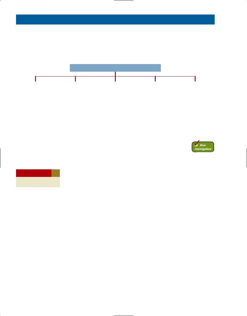
The organization and content of the chapter are as follows.
Reporting and Analyzing Receivables
|
Types of |
|
|
Accounts |
|
|
Notes |
|
|
Statement |
|
|
Managing |
|
|
|
|
|
|
|
Presentation of |
|
|
||||
|
Receivables |
|
|
Receivable |
|
|
Receivable |
|
|
|
|
Receivables |
|
|
|
|
|
|
|
|
Receivables |
|
|
||||
|
|
|
|
|
|
|
|
|
|
|
|
|
|
|
|
|
|
|
|
|
|
|
|
|
|
|
|
• |
Accounts receivable |
|
• |
Recognizing accounts |
|
• |
Determining the |
|
• |
Balance sheet and |
|
• |
Extending credit |
• |
Notes receivable |
|
|
receivable |
|
|
maturity date |
|
|
notes |
|
• |
Establishing a |
|
|
|
|
|
|
|
|
|
|
||||
• |
Other receivables |
|
• |
Valuing accounts |
|
• |
Computing interest |
|
• |
Income statement |
|
|
payment period |
|
|
receivable |
|
• |
Recognizing notes |
|
|
|
|
• |
Monitoring collections |
||
|
|
|
|
|
|
|
|
|
|||||
|
|
|
|
|
|
|
|
|
|
||||
|
|
|
|
|
|
|
receivable |
|
|
|
|
• |
Evaluating liquidity of |
|
|
|
|
|
|
|
|
|
|
|
|
||
|
|
|
|
|
|
• |
Valuing notes |
|
|
|
|
|
receivables |
|
|
|
|
|
|
|
receivable |
|
|
|
|
• |
Accelerating cash |
|
|
|
|
|
|
|
|
|
|
|
|
||
|
|
|
|
|
|
• |
Disposing of notes |
|
|
|
|
|
receipts |
|
|
|
|
|
|
|
receivable |
|
|
|
|
|
|
|
|
|
|
|
|
|
|
|
|
|
|
|
|
study objective 1
Identify the different types of receivables.
Types of Receivables
The term receivables refers to amounts due from individuals and companies. Receivables are claims that are expected to be collected in cash. The management of receivables is a very important activity for any company that sells goods or services on credit.
Receivables are important because they represent one of a company’s most liquid assets. For many companies, receivables are also one of the largest assets. For example, receivables represented 30.8% of the current assets of pharmaceutical giant Rite Aid in 2009. Illustration 8-1 lists receivables as a percentage of total assets for five other well-known companies in a recent year.
Illustration 8-1 |
|
|
|
Receivables as a |
Receivables as a |
|
|
|
|
|
Company |
|
Percentage of Total Assets |
|
percentage of assets |
|
|||
|
|
General Electric |
52% |
|
|
|
Ford Motor Company |
42% |
|
|
|
Minnesota Mining and Manufacturing Company |
|
|
|
|
(3M) |
14% |
|
|
|
DuPont Co. |
17% |
|
|
|
Intel Corporation |
5% |
|
|
|
|
|
|
The relative significance of a company’s receivables as a percentage of its assets depends on various factors: its industry, the time of year, whether it extends long-term financing, and its credit policies. To reflect important differences among receivables, they are frequently classified as (1) accounts receivable,
(2) notes receivable, and (3) other receivables.
Accounts receivable are amounts customers owe on account. They result from the sale of goods and services. Companies generally expect to collect
398

337
Accounts Receivable 399
accounts receivable within 30 to 60 days. They are usually the most significant type of claim held by a company.
Notes receivable represent claims for which formal instruments of credit are issued as evidence of the debt. The credit instrument normally requires the debtor to pay interest and extends for time periods of 60–90 days or longer. Notes and accounts receivable that result from sales transactions are often called trade receivables.
Other receivables include nontrade receivables such as interest receivable, loans to company officers, advances to employees, and income taxes refundable. These do not generally result from the operations of the business. Therefore, they are generally classified and reported as separate items in the balance sheet.
Ethics Note Companies report receivables from employees separately in the financial statements. The reason: Sometimes those assets are not the result of an “arm’s-length” transaction.
Accounts Receivable
Two accounting issues associated with accounts receivable are:
1.Recognizing accounts receivable.
2.Valuing accounts receivable.
A third issue, accelerating cash receipts from receivables, is discussed later in the chapter.
RECOGNIZING ACCOUNTS RECEIVABLE
Recognizing accounts receivable is relatively straightforward. A service organization records a receivable when it provides service on account. A merchandiser records accounts receivable at the point of sale of merchandise on account. When a merchandiser sells goods, it increases (debits) Accounts Receivable and increases (credits) Sales Revenue.
The seller may offer terms that encourage early payment by providing a discount. Sales returns also reduce receivables. The buyer might find some of the goods unacceptable and choose to return the unwanted goods.
To review, assume that Jordache Co. on July 1, 2012, sells merchandise on account to Polo Company for $1,000, terms 2/10, n/30. On July 5, Polo returns merchandise worth $100 to Jordache Co. On July 11, Jordache receives payment from Polo Company for the balance due. The journal entries to record these transactions on the books of Jordache Co. are as follows. (Cost of goods sold entries are omitted.)
study objective 2
Explain how accounts receivable are recognized in the accounts.
July |
1 |
|
|
Accounts Receivable—Polo Company |
|
|
1,000 |
|
|
|
|
|
Sales Revenue |
|
|
|
|
|
|
|
|
(To record sales on account) |
|
|
|
|
July |
5 |
|
|
Sales Returns and Allowances |
|
|
100 |
|
|
|
|
|
|||||
|
|
|
|
Accounts Receivable—Polo Company |
|
|
|
|
|
|
|
|
(To record merchandise returned) |
|
|
|
|
July 11 |
|
Cash ($900 $18) |
|
882 |
||||
|
|
|||||||
|
|
|
|
Sales Discounts ($900 .02) |
|
18 |
||
|
|
|
|
Accounts Receivable—Polo Company |
|
|
|
|
|
|
|
|
(To record collection of accounts |
|
|
|
|
|
|
|
|
receivable) |
|
|
|
|
|
|
|
|
|
|
|
||
1,000
Helpful Hint These entries are the same as those described in Chapter 5. For simplicity, we have
100omitted inventory and cost of goods sold from this set of journal entries and from end-of-chapter
material.
900
Some retailers issue their own credit cards. When you use a retailer’s credit card (JCPenney, for example), the retailer charges interest on the balance due if not paid within a specified period (usually 25–30 days).
To illustrate, assume that you use your JCPenney Company credit card to purchase clothing with a sales price of $300. JCPenney will increase (debit)

338
400 chapter 8 Reporting and Analyzing Receivables
A = L + SE
300
300 Rev
Cash Flows no effect
A = L + SE
4.50
4.50 Rev
Cash Flows no effect
Accounts Receivable for $300 and increase (credit) Sales Revenue for $300 (cost of goods sold entry omitted) as follows.
Accounts Receivable |
300 |
Sales Revenue |
300 |
(To record sale of merchandise) |
|
Assuming that you owe $300 at the end of the month, and JCPenney charges 1.5% per month on the balance due, the adjusting entry that JCPenney makes to record interest revenue of $4.50 ($300 1.5%) is as follows.
Accounts Receivable |
4.50 |
Interest Revenue |
4.50 |
(To record interest on amount due) |
|
Interest revenue is often substantial for many retailers.
ANATOMY OF A FRAU D
Tasanee was the accounts receivable clerk for a large non-profit foundation that provided performance and exhibition space for the performing and visual arts. Her responsibilities included activities normally assigned to an accounts receivable clerk, such as recording revenues from various sources that included donations, facility rental fees, ticket revenue, and bar receipts. However, she was also responsible for handling all cash and checks from the time they were received until the time she deposited them, as well as preparing the bank reconciliation. Tasanee took advantage of her situation by falsifying bank deposits and bank reconciliations so that she could steal cash from the bar receipts. Since nobody else logged the donations or matched the donation receipts to pledges prior to Tasanee receiving them, she was able to offset the cash that was stolen against donations that she received but didn’t record. Her crime was made easier by the fact that her boss, the company’s controller, only did a very superficial review of the bank reconciliation and thus didn’t notice that some numbers had been cut out from other documents and taped onto the bank reconciliation.
Total take: $1.5 million
THE MISSING CONTROLS
Segregation of duties. The foundation should not have allowed an accounts receivable clerk, whose job was to record receivables, to also handle cash, record cash, and make deposits, and especially prepare the bank reconciliation.
Independent internal verification. The controller was supposed to perform a thorough review of the bank reconciliation. Because he did not, he was terminated from his position.
Source: Adapted from Wells, Fraud Casebook (2007), pp. 183–194.
study objective 3
Describe the methods used to account for bad debts.
VALUING ACCOUNTS RECEIVABLE
Once companies record receivables in the accounts, the next question is: How should they report receivables in the financial statements? Companies report accounts receivable on the balance sheet as an asset. Determining the amount to report is sometimes difficult because some receivables will become uncollectible.
Although each customer must satisfy the credit requirements of the seller before the credit sale is approved, inevitably some accounts receivable become uncollectible. For example, a corporate customer may not be able to pay because it experienced a sales decline due to an economic downturn. Similarly, individuals may be laid off from their jobs or be faced with unexpected hospital bills. The seller

339
Accounts Receivable 401
records these losses that result from extending credit as Bad Debts Expense. Such losses are a normal and necessary risk of doing business on a credit basis.
Recently, when U.S. home prices fell, home foreclosures rose, and the economy in general slowed, lenders experienced huge increases in their bad debts expense. For example, during a recent quarter Wachovia, the fourth largest U.S. bank, increased bad debts expense from $108 million to $408 million. Similarly, American Express increased its bad debts expense by 70%.
The accounting profession uses two methods for uncollectible accounts: (1) the direct write-off method, and (2) the allowance method. We explain each of these methods in the following sections.
Direct Write-Off Method for Uncollectible Accounts
Under the direct write-off method, when a company determines receivables from a particular company to be uncollectible, it charges the loss to Bad Debts Expense. Assume, for example, that Warden Co. writes off M. E. Doran’s $200 balance as uncollectible on December 12. Warden’s entry is:
Dec. 12 |
|
Bad Debts Expense |
200 |
|
|
|
Accounts Receivable—M. E. Doran |
|
200 |
|
|
(To record write-off of M. E. Doran |
|
|
|
|
account) |
|
|
|
|
|
Under this method, bad debts expense will show only actual losses from uncollectibles. The company reports accounts receivable at its gross amount without any adjustment for estimated losses for bad debts.
Use of the direct write-off method can reduce the usefulness of both the income statement and balance sheet. Consider the following example. In 2012, Quick Buck Computer Company decided it could increase its revenues by offering computers to college students without requiring any money down, and with no creditapproval process. It went on campuses across the country and sold one million computers at a selling price of $800 each. This promotion increased Quick Buck’s revenues and receivables by $800,000,000. It was a huge success: The 2012 balance sheet and income statement looked wonderful. Unfortunately, during 2013, nearly 40% of the college student customers defaulted on their loans. The 2013 income statement and balance sheet looked terrible. Illustration 8-2 shows the effect of these events on the financial statements using the direct write-off method.
Alternative Terminology You will sometimes see Bad Debts Expense called Uncollectible Accounts Expense.
A = L + SE
200 Exp
200
Cash Flows no effect
Illustration 8-2 Effects
Year 2012 |
Year 2013 |
of direct write-off method |
|
|
|
Net |
Net |
|
income |
income |
|
Huge sales promotion. |
Customers default on loans. |
|
Sales increase dramatically. |
Bad debts expense increases dramatically. |
|
Accounts receivable increases dramatically. |
Accounts receivable plummets. |
|
Under the direct write-off method, companies often record bad debts expense in a period different from the period in which they recorded the revenue. Thus, no attempt is made to match bad debts expense to sales revenues in the income statement. Nor does the company try to show accounts receivable in the balance sheet at the amount actually expected to be received. Consequently, unless a company expects bad debts losses to be insignificant, the direct write-off method is not acceptable for financial reporting purposes.