310
preview of chapter 6
In the previous chapter, we discussed the accounting for merchandise inventory using a perpetual inventory system. In this chapter, we explain the methods used to calculate the cost of inventory on hand at the balance sheet date and the cost of goods sold. We conclude by illustrating methods for analyzing inventory.
The content and organization of this chapter are as follows.
Reporting and Analyzing Inventory
|
Classifying Inventory |
|
Determining |
|
|
Inventory Quantities |
|
|
|
|
|
|
|
• |
Merchandising |
|
• Taking a physical inventory |
• |
Manufacturing |
|
• Determining ownership of |
• |
Just-in-time |
|
goods |
|
|
|
|
|
|
|
Inventory Costing |
|
|
Analysis of Inventory |
|
|
|
|
|
• |
Specific identification |
|
• |
Inventory turnover ratio |
• |
Cost flow assumptions |
|
• |
LIFO reserve |
•Financial statement and tax effects
•Consistent use
•Lower-of-cost-or-market
Helpful Hint Regardless of the classification, companies report all inventories under Current Assets on the balance sheet.
Classifying Inventory
How a company classifies its inventory depends on whether the firm is a merchandiser or a manufacturer. In a merchandising company, such as those described in Chapter 5, inventory consists of many different items. For example, in a grocery store, canned goods, dairy products, meats, and produce are just a few of the inventory items on hand. These items have two common characteristics: (1) They are owned by the company, and (2) they are in a form ready for sale to customers in the ordinary course of business. Thus, merchandisers need only one inventory classification, merchandise inventory, to describe the many different items that make up the total inventory.
In a manufacturing company, some inventory may not yet be ready for sale. As a result, manufacturers usually classify inventory into three categories: finished goods, work in process, and raw materials. Finished goods inventory is manufactured items that are completed and ready for sale. Work in process is that portion of manufactured inventory that has begun the production process but is not yet complete. Raw materials are the basic goods that will be used in production but have not yet been placed into production.
For example, Caterpillar classifies earth-moving tractors completed and ready for sale as finished goods. It classifies the tractors on the assembly line in various stages of production as work in process. The steel, glass, tires, and other components that are on hand waiting to be used in the production of tractors are identified as raw materials.
The accounting concepts discussed in this chapter apply to the inventory classifications of both merchandising and manufacturing companies. Our focus throughout most of this chapter is on merchandise inventory.
By observing the levels and changes in the levels of these three inventory types, financial statement users can gain insight into management’s production plans. For example, low levels of raw materials and high levels of finished goods suggest that management believes it has enough inventory on hand, and production will be slowing down—perhaps in anticipation of a recession. On the other hand, high levels of raw materials and low levels of finished goods probably indicate that management is planning to step up production.
311
Determining Inventory Quantities 283
Many companies have significantly lowered inventory levels and costs using just-in-time (JIT) inventory methods. Under a just-in-time method, companies manufacture or purchase goods just in time for use. Dell is famous for having developed a system for making computers in response to individual customer requests. Even though it makes computers to meet a customer’s particular specifications, Dell is able to assemble the computer and put it on a truck in less than 48 hours. The success of a JIT system depends on reliable suppliers. By integrating its information systems with those of its suppliers, Dell reduced its inventories to nearly zero. This is a huge advantage in an industry where products become obsolete nearly overnight.
Accounting Across the Organization
A Big Hiccup
JIT can save a company a lot of money, but it isn’t without risk. An unexpected disruption in the supply chain can cost a company a lot of money. Japanese automakers experienced just such a disruption when a 6.8-magnitude earthquake caused major damage to the company that produces 50% of their piston rings. The rings themselves cost only $1.50, but without them you cannot make a car. No other supplier could quickly begin producing sufficient quantities of the rings to match the desired specifications. As a result, the automakers were forced to shut down production for a few days—a loss of tens of thousands of cars.
Source: Amy Chozick, “A Key Strategy of Japan’s Car Makers Backfires,” Wall Street Journal (July 20, 2007).
?What steps might the companies take to avoid such a serious disruption in the future? (See page 330.)
Determining Inventory Quantities
No matter whether they are using a periodic or perpetual inventory system, all companies need to determine inventory quantities at the end of the accounting period. If using a perpetual system, companies take a physical inventory for two purposes: The first purpose is to check the accuracy of their perpetual inventory records. The second is to determine the amount of inventory lost due to wasted raw materials, shoplifting, or employee theft.
Companies using a periodic inventory system must take a physical inventory for two different purposes: to determine the inventory on hand at the balance sheet date, and to determine the cost of goods sold for the period.
Determining inventory quantities involves two steps: (1) taking a physical inventory of goods on hand and (2) determining the ownership of goods.
TAKING A PHYSICAL INVENTORY
Companies take the physical inventory at the end of the accounting period. Taking a physical inventory involves actually counting, weighing, or measuring each kind of inventory on hand. In many companies, taking an inventory is a formidable task. Retailers such as Target, True Value Hardware, or Home Depot have thousands of different inventory items. An inventory count is generally more accurate when a limited number of goods are being sold or received during the counting. Consequently, companies often “take inventory” when the business is closed or when business is slow. Many retailers close early on a chosen day in January—after the holiday sales and returns, when inventories are at their lowest level—to count inventory. Recall from Chapter 5 that Wal-Mart had a yearend of January 31.
study objective 1
Describe the steps in determining inventory quantities.
Ethics Note In a famous fraud, a salad oil company filled its storage tanks mostly with water. The oil rose to the top, so auditors thought the tanks were full of oil. The company also said it had more tanks than it really did: it repainted numbers on the tanks to confuse auditors.
312
284 chapter 6 Reporting and Analyzing Inventory
Ethics Insight
Falsifying Inventory to Boost Income
Managers at women’s apparel maker Leslie Fay were convicted of falsifying inventory records to boost net income—and consequently to boost management bonuses. In another case, executives at Craig Consumer Electronics were accused of defrauding lenders by manipulating inventory records. The indictment said the company classified “defective goods as new or refurbished” and claimed that it owned certain shipments “from overseas suppliers” when, in fact, Craig either did not own the shipments or the shipments did not exist.
?What effect does an overstatement of inventory have on a company’s financial statements? (See page 330.)
DETERMINING OWNERSHIP OF GOODS
One challenge in determining inventory quantities is making sure a company owns the inventory. To determine ownership of goods, two questions must be answered: Do all of the goods included in the count belong to the company? Does the company own any goods that were not included in the count?
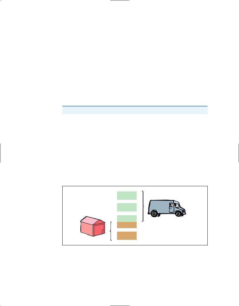
Goods in Transit
A complication in determining ownership is goods in transit (on board a truck, train, ship, or plane) at the end of the period. The company may have purchased goods that have not yet been received, or it may have sold goods that have not yet been delivered. To arrive at an accurate count, the company must determine ownership of these goods.
Goods in transit should be included in the inventory of the company that has legal title to the goods. Legal title is determined by the terms of the sale, as shown in Illustration 6-1 and described below.
Illustration 6-1 |
Terms of |
|
|
sale |
|
|
|
|
|
|
FOB Shipping Point |
|
FOB Destination |
Ownership |
Buyer pays freight costs |
|
Seller pays freight costs Ownership |
passes to |
|
|
|
passes to |
buyer here |
|
|
buyer here |
|
|
Public |
|
Public |
|
|
Carrier |
|
Carrier |
Seller |
|
Co. |
Seller |
Co. |
|
Buyer |
Buyer |
1.When the terms are FOB (free on board) shipping point, ownership of the goods passes to the buyer when the public carrier accepts the goods from the seller.
2.When the terms are FOB destination, ownership of the goods remains with the seller until the goods reach the buyer.
Consigned Goods
In some lines of business, it is common to hold the goods of other parties and try to sell the goods for them for a fee, but without taking ownership of the goods. These are called consigned goods.
For example, you might have a used car that you would like to sell. If you take the item to a dealer, the dealer might be willing to put the car on its lot and
Do it!
313
Determining Inventory Quantities 285
charge you a commission if it is sold. Under this agreement, the dealer would not take ownership of the car, which would still belong to you. If an inventory count were taken, the car would not be included in the dealer’s inventory because the dealer does not own it.
Many car, boat, and antique dealers sell goods on consignment to keep their inventory costs down and to avoid the risk of purchasing an item that they won’t be able to sell. Today, even some manufacturers are making consignment agreements with their suppliers in order to keep their inventory levels low.
before you go on...
 Hasbeen Company completed its inventory count. It arrived at a total inventory value of $200,000. You have been given the information listed below. Discuss how this information affects the reported cost of inventory.
1.Hasbeen included in the inventory goods held on consignment for Falls Co., costing $15,000.
2.The company did not include in the count purchased goods of $10,000, which were in transit (terms: FOB shipping point).
3.The company did not include in the count inventory that had been sold with a cost of
$12,000, which was in transit (terms: FOB shipping point).
Solution
The goods of $15,000 held on consignment should be deducted from the inventory count. The goods of $10,000 purchased FOB shipping point should be added to the inventory count. Sold goods of $12,000 which were in transit FOB shipping point should not be included in the ending inventory. Inventory should be $195,000 ($200,000 $15,000 $10,000).
Related exercise material: BE6-1, Do it! 6-1, E6-1, E6-2, and E6-3.
RULES OF OWNERSHIP
Action Plan
•Apply the rules of ownership to goods held on consignment.
•Apply the rules of ownership to goods in transit.
A N ATO M Y O F A F R AU D
Ted Nickerson, CEO of clock manufacturer Dally Industries, was feared by all of his employees. Ted had expensive tastes. To support his expensive tastes, Ted took out large loans, which he collateralized with his shares of Dally Industries stock. If the price of Dally’s stock fell, he was required to provide the bank with more shares of stock. To achieve target net income figures and thus maintain the stock price, Ted coerced employees in the company to alter inventory figures. Inventory quantities were manipulated by changing the amounts on inventory control tags after the year-end physical inventory count. For example, if a tag said there were 20 units of a particular item, the tag was changed to 220. Similarly, the unit costs that were used to determine the value of ending inventory were increased from, for example, $125 per unit to $1,250. Both of these fraudulent changes had the effect of increasing the amount of reported ending inventory. This reduced cost of goods sold and increased net income.
Total take: $245,000
THE MISSING CONTROL
Independent internal verification. The company should have spot-checked its inventory records periodically, verifying that the number of units in the records agreed with the amount on hand and that the unit costs agreed with vendor price sheets.
Source: Adapted from Wells, Fraud Casebook (2007), pp. 502–509.
314
286 chapter 6 Reporting and Analyzing Inventory
study objective 2
Explain the basis of accounting for inventories and apply the inventory cost flow methods under a periodic inventory system.
Inventory Costing
Inventory is accounted for at cost. Cost includes all expenditures necessary to acquire goods and place them in a condition ready for sale. For example, freight costs incurred to acquire inventory are added to the cost of inventory, but the cost of shipping goods to a customer are a selling expense. After a company has determined the quantity of units of inventory, it applies unit costs to the quantities to determine the total cost of the inventory and the cost of goods sold. This process can be complicated if a company has purchased inventory items at different times and at different prices.
For example, assume that Crivitz TV Company purchases three identical 50inch TVs on different dates at costs of $700, $750, and $800. During the year, Crivitz sold two sets at $1,200 each. These facts are summarized in Illustration 6-2.
|
Illustration 6-2 Data for |
Purchases |
|
|
|
|
|
inventory costing example |
|
|
|
|
|
Feb. 3 |
1 |
TV |
at |
$700 |
|
|
|
|
March 5 |
1 |
TV |
at |
$750 |
|
|
May 22 |
1 |
TV |
at |
$800 |
|
|
Sales |
|
|
|
|
|
|
June 1 |
2 |
TVs |
for |
$2,400 ($1,200 2) |
|
|
|
|
|
|
|
Illustration 6-3 Specific identification method
Cost of goods sold will differ depending on which two TVs the company sold. For example, it might be $1,450 ($700 $750), or $1,500 ($700 $800), or $1,550 ($750 $800). In this section, we discuss alternative costing methods available to Crivitz.
SPECIFIC IDENTIFICATION
If Crivitz can positively identify which particular units it sold and which are still in ending inventory, it can use the specific identification method of inventory costing. For example, if Crivitz sold the TVs it purchased on February 3 and May 22, then its cost of goods sold is $1,500 ($700 $800), and its ending inventory is $750 (see Illustration 6-3). Using this method, companies can accurately determine ending inventory and cost of goods sold.
|
SOLD |
Ending |
SOLD |
|
Inventory |
|
|
|
|
|
$700 |
|
$750 |
$800 |
Cost of goods sold = $700 + $800 = $1,500 |
|
|
Ending inventory = $750 |
Ethics Note A major disadvantage of the specific identification method is that management may be able to manipulate net income. For example, it can boost net income by selling units purchased at a low cost, or reduce net income by selling units purchased at a high cost.
Specific identification requires that companies keep records of the original cost of each individual inventory item. Historically, specific identification was possible only when a company sold a limited variety of high-unit-cost items that could be identified clearly from the time of purchase through the time of sale. Examples of such products are cars, pianos, or expensive antiques.
Today, with bar coding, electronic product codes, and radio frequency identification, it is theoretically possible to do specific identification with nearly any type of product. The reality is, however, that this practice is still relatively rare. Instead, rather than keep track of the cost of each particular item sold, most companies make assumptions, called cost flow assumptions, about which units were sold.
315
Inventory Costing 287
COST FLOW ASSUMPTIONS
Because specific identification is often impractical, other cost flow methods are permitted. These differ from specific identification in that they assume flows of costs that may be unrelated to the actual physical flow of goods. There are three assumed cost flow methods:
1.First-in, first-out (FIFO)
2.Last-in, first-out (LIFO)
3.Average-cost
There is no accounting requirement that the cost flow assumption be consistent with the physical movement of the goods. Company management selects the appropriate cost flow method.
To demonstrate the three cost flow methods, we will use a periodic inventory system. We assume a periodic system for two main reasons. First, many small companies use periodic rather than perpetual systems. Second, very few companies use perpetual LIFO, FIFO, or average-cost to cost their inventory and related cost of goods sold. Instead, companies that use perpetual systems often use an assumed cost (called a standard cost) to record cost of goods sold at the time of sale. Then, at the end of the period when they count their inventory, they recalculate cost of goods sold using periodic FIFO, LIFO, or averagecost and adjust cost of goods sold to this recalculated number.1
To illustrate the three inventory cost flow methods, we will use the data for Houston Electronics’ Astro condensers, shown in Illustration 6-4.
HOUSTON ELECTRONICS
Astro Condensers
|
Date |
|
Explanation |
Units |
|
Unit Cost |
Total Cost |
|
|
|
|
|
|
|
|
|
|
|
|
|
|
Jan. 1 |
|
Beginning inventory |
100 |
$10 |
|
$ 1,000 |
|
|
Apr. 15 |
|
Purchase |
200 |
11 |
|
2,200 |
|
|
Aug. 24 |
|
Purchase |
300 |
12 |
|
3,600 |
|
|
Nov. 27 |
|
Purchase |
|
400 |
13 |
|
|
5,200 |
|
|
|
|
|
Total units available for sale |
1,000 |
|
|
|
$12,000 |
|
|
|
|
|
Units in ending inventory |
450 |
|
|
|
|
|
|
|
|
|
|
|
|
|
|
|
|
|
|
|
|
|
|
|
|
|
Units sold |
550 |
|
|
|
|
|
|
|
|
|
|
|
|
|
|
|
|
|
|
|
|
|
|
Illustration 6-4 Data for Houston Electronics
From Chapter 5, the cost of goods sold formula in a periodic system is:
(Beginning Inventory Purchases) Ending Inventory Cost of Goods Sold
Houston Electronics had a total of 1,000 units available to sell during the period (beginning inventory plus purchases). The total cost of these 1,000 units is $12,000, referred to as cost of goods available for sale. A physical inventory taken at December 31 determined that there were 450 units in ending inventory. Therefore, Houston sold 550 units (1,000 450) during the period. To determine the cost of the 550 units that were sold (the cost of goods sold), we assign a cost to the ending inventory and subtract that value from the cost of goods available for sale. The
1Also, some companies use a perpetual system to keep track of units, but they do not make an entry for perpetual cost of goods sold. In addition, firms that employ LIFO tend to use dollarvalue LIFO, a method discussed in upper-level courses. FIFO periodic and FIFO perpetual give the same result; therefore firms should not incur the additional cost to use FIFO perpetual. Few firms use perpetual average-cost because of the added cost of record-keeping. Finally, for instructional purposes, we believe it is easier to demonstrate the cost flow assumptions under the periodic system, which makes it more pedagogically appropriate.
316
288 chapter 6 Reporting and Analyzing Inventory
Illustration 6-5 Allocation of costs—FIFO method
Helpful Hint Note the sequencing of the allocation: (1) Compute ending inventory, and (2) determine cost of goods sold.
value assigned to the ending inventory will depend on which cost flow method we use. No matter which cost flow assumption we use, though, the sum of cost of goods sold plus the cost of the ending inventory must equal the cost of goods available for sale—in this case, $12,000.
First-In, First-Out (FIFO)
The FIFO (first-in, first-out) method assumes that the earliest goods purchased are the first to be sold. FIFO often parallels the actual physical flow of merchandise because it generally is good business practice to sell the oldest units first. Under the FIFO method, therefore, the costs of the earliest goods purchased are the first to be recognized in determining cost of goods sold, regardless which units were actually sold. (Note that this does not mean that the oldest units are sold first, but that the costs of the oldest units are recognized first. In a bin of picture hangers at the hardware store, for example, no one really knows, nor would it matter, which hangers are sold first.) Illustration 6-5 shows the allocation of the cost of goods available for sale at Houston Electronics under FIFO.
COST OF GOODS AVAILABLE FOR SALE
|
Date |
Explanation |
|
Units |
Unit Cost |
|
Total Cost |
|
Jan. 1 |
Beginning inventory |
|
100 |
|
$10 |
|
$ |
1,000 |
|
|
Apr. 15 |
Purchase |
200 |
11 |
|
|
|
2,200 |
|
|
Aug. 24 |
Purchase |
300 |
12 |
|
|
|
3,600 |
|
|
Nov. 27 |
Purchase |
400 |
13 |
|
|
|
5,200 |
|
|
|
|
|
|
|
|
|
|
|
|
|
|
|
Total |
1,000 |
|
|
$12,000 |
|
|
|
|
|
|
|
|
|
|
|
|
|
|
|
|
|
|
|
|
|
|
|
|
|
|
|
|
|
Helpful Hint Another way of thinking about the calculation of FIFO ending inventory is the
LISH assumption—last in still here.
|
STEP 1: ENDING INVENTORY |
STEP 2: COST OF GOODS SOLD |
|
|
|
|
|
|
|
|
|
|
|
|
|
|
|
|
|
|
|
|
|
|
|
|
|
Unit |
|
Total |
|
|
|
|
|
Date |
Units |
Cost |
|
Cost |
|
|
|
|
|
|
|
|
|
|
|
|
|
|
|
|
|
|
|
|
|
Nov. 27 |
400 |
|
|
|
$13 |
|
$ 5,200 |
Cost of goods available for sale |
$12,000 |
|
Aug. 24 |
50 |
|
|
12 |
|
|
600 |
Less: Ending inventory |
5,800 |
|
|
|
|
|
|
|
|
|
|
|
|
|
|
|
|
Total |
450 |
|
|
|
|
|
$5,800 |
Cost of goods sold |
$ 6,200 |
|
|
|
|
|
|
|
|
|
|
|
|
|
|
|
|
|
$1,000 |
Cost of |
goods sold |
$2,200 |
$6,200 |
|
$3,000 |
|
$600 |
|
Warehouse
$5,200
Ending inventory
Under FIFO, since it is assumed that the first goods purchased were the first goods sold, ending inventory is based on the prices of the most recent units purchased. That is, under FIFO, companies determine the cost of the ending inventory by taking the unit cost of the most recent purchase and working backward until all units of inventory have been costed. In this example, Houston Electronics prices the 450 units of ending inventory using the most recent prices. The last purchase was 400 units at $13 on November 27. The remaining 50 units are priced using the unit cost of the second most recent
318
290 chapter 6 Reporting and Analyzing Inventory
Illustration 6-8 Proof of cost of goods sold
Under LIFO, since it is assumed that the first goods sold were those that were most recently purchased, ending inventory is based on the prices of the oldest units purchased. That is, under LIFO, companies obtain the cost of the ending inventory by taking the unit cost of the earliest goods available for sale and working forward until all units of inventory have been costed. In this example, Houston Electronics prices the 450 units of ending inventory using the earliest prices. The first purchase was 100 units at $10 in the January 1 beginning inventory. Then 200 units were purchased at $11. The remaining 150 units needed are priced at $12 per unit (August 24 purchase). Next, Houston Electronics calculates cost of goods sold by subtracting the cost of the units not sold (ending inventory) from the cost of all goods available for sale.
Illustration 6-8 demonstrates that we can also calculate cost of goods sold by pricing the 550 units sold using the prices of the last 550 units acquired. Note that of the 300 units purchased on August 24, only 150 units are assumed sold. This agrees with our calculation of the cost of ending inventory, where 150 of these units were assumed unsold and thus included in ending inventory.
|
Date |
|
Units |
Unit Cost |
Total Cost |
|
|
|
|
|
|
|
|
|
|
|
|
|
|
Nov. 27 |
400 |
|
|
$13 |
|
$ 5,200 |
|
|
Aug. 24 |
150 |
|
|
12 |
|
|
1,800 |
|
|
|
|
|
|
|
|
|
|
|
|
|
|
|
|
Total |
550 |
|
|
|
|
$7,000 |
|
|
|
|
|
|
|
|
|
|
|
|
|
|
|
|
|
|
|
|
|
|
|
|
|
|
|
|
|
|
|
|
|
Illustration 6-9 Formula for weighted-average unit cost
Under a periodic inventory system, which we are using here, all goods purchased during the period are assumed to be available for the first sale, regardless of the date of purchase.
Average-Cost
The average-cost method allocates the cost of goods available for sale on the basis of the weighted-average unit cost incurred. Illustration 6-9 presents the formula and a sample computation of the weighted-average unit cost.
Cost of Goods |
|
Total Units |
|
Weighted- |
Available |
|
Available |
|
Average |
for Sale |
|
for Sale |
|
Unit Cost |
$12,000 |
|
1,000 |
|
$12.00 |
|
|
|
|
|
The company then applies the weighted-average unit cost to the units on hand to determine the cost of the ending inventory. Illustration 6-10 shows the allocation of the cost of goods available for sale at Houston Electronics using average-cost.
We can verify the cost of goods sold under this method by multiplying the units sold times the weighted-average unit cost (550 $12 $6,600). Note that this method does not use the simple average of the unit costs. That average is $11.50 ($10 $11 $12 $13 $46; $46 4). The average-cost method instead uses the average weighted by the quantities purchased at each unit cost.
319
|
|
|
|
|
|
|
|
|
|
|
|
|
|
Inventory Costing 291 |
|
|
|
|
|
|
|
|
|
|
|
|
|
|
Illustration 6-10 |
|
|
|
COST OF GOODS AVAILABLE FOR SALE |
|
|
|
|
|
|
|
|
|
|
|
|
|
|
|
Allocation of costs— |
|
|
|
|
|
|
|
|
|
|
|
|
|
|
average-cost method |
|
Date |
|
Explanation |
|
Units |
Unit Cost |
|
Total Cost |
|
|
|
|
|
|
|
|
|
|
|
|
|
|
|
|
|
|
|
|
Jan. 1 |
Beginning inventory |
100 |
$10 |
$ |
1,000 |
|
|
|
Apr. 15 |
Purchase |
200 |
11 |
|
|
|
2,200 |
|
|
|
Aug. 24 |
Purchase |
300 |
12 |
|
|
|
3,600 |
|
|
|
Nov. 27 |
Purchase |
400 |
13 |
|
|
|
5,200 |
|
|
|
|
|
|
|
|
|
|
|
|
|
|
|
|
|
Total |
1,000 |
|
|
$12,000 |
|
|
|
|
|
|
|
|
|
|
|
|
|
|
|
|
|
|
|
|
|
|
|
|
|
|
|
|
|
|
|
|
|
STEP 1: ENDING INVENTORY |
|
STEP 2: COST OF GOODS SOLD |
|
|
|
|
|
|
|
|
|
|
|
|
|
|
|
|
$12,000 |
1,000 |
|
$12.00 |
|
|
Unit |
|
Total |
Units |
|
Cost |
|
|
Cost |
450 |
$12.00 |
$5,400 |
|
|
|
|
|
|
|
|
|
|
|
|
Cost of goods available for sale |
$12,000 |
Less: Ending inventory |
|
5,400 |
Cost of goods sold |
$ 6,600 |
|
|
|
$12,000
––––––––– = $12 per unit 1,000 units
Cost per unit
|
450 |
× $12 |
|
|
units |
Warehouse |
|
|
|
= |
|
|
|
$5,400 |
|
Ending inventory
$12,000 – $5,400 = $6,600
Cost of goods sold
Do it! The accounting records of Shumway Ag Implement show the following data.
Beginning inventory |
4,000 units at $3 |
Purchases |
6,000 units at $4 |
Sales |
7,000 units at $12 |
Determine (a) the cost of goods available for sale and (b) the cost of goods sold during the period under a periodic system using (i) FIFO, (ii) LIFO, and (iii) average-cost.
Solution
(a)Cost of goods available for sale: (4,000 $3) (6,000 $4) $36,000
(b)Cost of goods sold using:
(i)FIFO: $36,000 (3,000* $4) $24,000
(ii)LIFO: $36,000 (3,000 $3) $27,000
(iii)Average-cost: Weighted-average price ($36,000 10,000) $3.60 $36,000 (3,000 $3.60) $25,200
*(4,000 6,000 7,000)
COST FLOW METHODS
Action Plan
•Understand the periodic inventory system.
•Allocate costs between goods sold and goods on hand (ending inventory) for each cost flow method.
•Compute cost of goods sold for each cost flow method.
Related exercise material: BE6-2, BE6-3, Do it! 6-2, E6-4, and E6-5.