3. Статья NIPE_WP_19_2009

“ Fundamentals, Financial Factors and The Dynamics of

Investment in Emerging Markets”

Tuomas A. Peltonen

Ricardo M. Sousa

Isabel S. Vansteenkiste

NIPE* WP 19/2009

URL:

http://www.eeg.uminho.pt/economia/nipe

* NIPE – Núcleo de Investigação em Políticas Económicas – is supported by the Portuguese Foundation for Science and Technology through the Programa Operacional Ciência, Teconologia e Inovação (POCI 2010) of the

Quadro Comunitário de Apoio III, which is financed by FEDER and Portuguese funds.

Fundamentals, Financial Factors and

The Dynamics of Investment in Emerging Markets

Abstract

The paper uses a Panel Vector Auto-Regression (PVAR) approach to analyze the shortrun adjustment of private investment to shocks to fundamental and …nancial factors in emerging market economies.

By relying on a panel of 31 emerging economies and quarterly frequency data for the period 1990:1-2008:3, we show that: (i) investment sluggishly adjusts to its own shocks; (ii) GDP and equity price shocks have a positive and sizeable impact on investment; (iii) unexpected variation in the cost of capital and the lending rate has a negative (although economically small) e¤ect on investment; and (iv) the response of investment to credit market developments seems to be driven by the demand side.

In addition, the empirical evidence suggests that the e¤ects of equity price shocks are similar for emerging Asia and Latin America, but credit shocks are more important in Latin America. Moreover, shocks to the lending rate have a very pronounced and negative impact in emerging European markets.

Finally, we show that the stock market bubbles may have encouraged real investment during the nineties.

Keywords: fundamentals, …nancial factors, investment, emerging markets, panel VAR.

JEL Classi…cation: E22, E44, D24.

The authors would like to thank Marcel Fratzscher, Andrew Rose, Roland Straub, Shang-Jin Wei, an anonymous referee and seminar participants at the ECB for useful comments. The code used to estimate the panel VAR model is a modi…cation of the program provided by Inessa Love and Lea Ziccino and is based on Love, I., and L. Zicchino (2006). Financial development and dynamic investment behavior: evidence from panel VAR. The Quarterly Review of Economics and Finance, 46(2), 190-210.

yEuropean Central Bank, Kaiserstraß 29, D-60311 Frankfurt am Main, Germany. Email: tuomas.peltonen@ecb.europa.eu.

zCorresponding author. University of Minho, Department of Economics and Economic Policies Research Unit (NIPE), Campus of Gualtar, 4710-057 - Braga, Portugal; London School of Economics, Financial Markets Group (FMG), Houghton Street, London WC2 2AE, United Kingdom. European Central Bank, Kaiserstraß 29, D-60311 Frankfurt am Main, Germany. Email: rjsousa@eeg.uminho.pt, rjsousa@alumni.lse.ac.uk. Ricardo Sousa would like to thank the International Policy Analysis and Emerging Markets Division of the ECB for its hospitality.

xEuropean Central Bank, Kaiserstraß 29, D-60311 Frankfurt am Main, Germany. Email: isabel.vansteenkiste@ecb.europa.eu.

1

1Introduction

Private investment is a critical determinant of long-run economic performance, being pivotal to a country’s economic growth and employment situation. For emerging market economies, private investment is particularly relevant as it contributes to their catching-up process with advanced countries. In fact, despite the wide di¤erences across countries,1 private investment represented, on average, 20-25% of GDP in emerging countries over the period 1990-2007.

While the role of private investment is unquestionable, there is surprisingly little research on its determinants in emerging market economies, a fact that can not be detached from the scarcity of data.

Moreover, the distinction between the "fundamental" and the "…nancial" determinants of investment remains important. In fact, despite the popularity of the neoclassical model, there is a growing literature that emphasizes the role played by …nancial constraints - namely, via interest rates and credit - on investment in emerging markets (McKinnon, 1973; Shaw, 1974; Fry, 1980; Sundararajan and Thakur, 1980; Tun Wai and Wong, 1982; Tybout, 1983; Blejer and Khan, 1984; O’Brien and Browne, 1992; Serven and Solimano, 1992; Whited, 1992; Harris et al., 1994; Jaramillo et al., 1996; Demirguc-Kunt and Maksimovic, 1998; Rajan and Zingales, 1998; Wurgler, 2000).

More recently, Peltonen et al. (2009) provide an attempt to uncover the long-run determinants of private investment growth in emerging markets. The authors show that: (i) the GDP and the cost of capital are among the "fundamental" determinants of investment; (ii) the equity price impacts positively and signi…cantly on investment; (iii) "…nancial" factors (such as, credit and lending rate) play an important role on the dynamics of investment, in particular, for emerging Asia and Latin America; (iv) investment growth exhibits substantial persistence; and (v) crises episodes magnify the negative response of investment.

The current …nancial turmoil and the extreme volatility of private investment have, however, brought to the …rst stage other similarly important policy questions: What explains the short-run dynamics of private investment in emerging markets? What are the likely e¤ects of unexpected variation in "fundamental" and "…nancial" determinants? How large are their impact and for how long do they persistent?

These are important issues, particularly, if one takes into account that part of the solution to the exit of the current crisis lies on the economic performance of emerging market economies given its increasing role in the world economy. Moreover, they lack a clear answer which we try to tackle with the current work.

In this paper, we use a Panel Vector Autoregression (PVAR) approach aimed at analyzing the short-run adjustment of investment to shocks to "fundamental" and "…nancial" factors in emerging market economies. We build a panel of 31 emerging economies using quarterly frequency data for the period 1990:1-2008:3, and show that: (i) investment shocks are, in general, persistent; (ii) GDP shocks have a positive and sizeable e¤ect on investment, re‡ecting the strong co-movement between the two macroeconomic aggregates; (iii) similarly, shocks to the equity price impact positively on investment, supporting the Tobin’s Q approach; (iv) in contrast, the cost of capital a¤ects negatively investment, although the magnitude of the e¤ect is small; and (v) the response of investment to a shock in credit is, in general, negative, suggesting that credit demand shocks (as opposed to credit supply shocks) play the dominant

1 A few countries, in particular the large emerging Asian markets, exhibit very high rates of private investment, exceeding 30%. At the other extreme, Brazil and the Philippines experience much lower rates of private investment, falling below 20% of GDP.

2

role.

Our …ndings are robust to the exclusion of the equity price index, to the replacement of credit by a monetary aggregate, and are not biased due to the occurrence of crises episodes.

In addition, the empirical …ndings suggest that the e¤ects of equity price shocks (on investment) are of similar magnitude in emerging Asia and Latin America, but credit shocks are more important in Latin America. Moreover, shocks to the lending rate have a very pronounced and negative impact in emerging European markets, re‡ecting the fact that these economies tend to be bank-based.

Finally, we show that the impact of the equity price on investment was stronger in the …rst half of the sample, that is, 1990:1-1999:4, a period characterized by a strong boom of stock markets. While this suggests that access to equity markets may actually amplify investment growth, it also poses important challenges to emerging markets, in particular, in the outcome of a downturn of …nancial markets.

The rest of the paper is organized as follows. Section 2 reviews the existing literature on the fundamental and …nancial factors determining private investment. Section 3 presents the estimation methodology and Section 4 describes the data. Section 5 discusses the empirical results and Section 6 provides the sensitivity analysis. Finally, Section 7 concludes with the main …ndings and policy implications.

2A Brief Review of the Literature

Two models describing the "fundamental" determinants of private investment often compete in the literature: (i) the traditional neoclassical model, i.e., the Jorgenson (1963) approach; and (ii) the alternative Q approach by Tobin (1969).

According to the Jorgenson approach investment can be modelled as the joint process of investment, output and the cost of capital. While the Jorgenson approach is still widely used by those who forecast investment using models of systems of equations, it has been rejected by most theorists (Lucas, 1976).

In the Q approach, investment is seen as the joint process with the Tobin’s Q ratio, that is, the ratio of the market valuation of a …rm’s securities to the replacement cost of the physical assets they represent (Brainard and Tobin, 1968). This ratio is an indicator of future pro…tability that combines asset prices in a su¢ cient statistic: stock prices, bond prices, and the replacement cost of the capital stock (Fischer and Merton, 1984).

There are a number of reasons to believe that stock prices may in‡uence investment: (i) when the market value of an additional unit of capital exceeds its replacement cost, a …rm can raise its pro…t by investing (Tobin, 1969; Von Furstenberg, 1977; Doan et al., 1984; Barro, 1990; Galeotti and Schiantarelli, 1994); (ii) a rise in stock prices improves the balance sheet position of the …rm (Bernanke and Gertler, 1989; Tease, 1993), which reduces the cost of capital (Fischer and Merton, 1984) and/or increases the availability of external funding (Bernanke and Gertler, 1989); and (iii) if the role of management is to maximize the wealth of existing shareholders, then investment should respond to stock prices even when they deviates from the true value of the …rm.

In contrast, another strand of the literature rejects the Q approach (Barro, 1990; Sensenbrenner, 1991) and considers that there is a minor role for stock prices beyond their ability to predict fundamental determinants of investment (Morck et al., 1990; Blanchard et al., 1993; Andersen and Subbaraman, 1996; Chirinko and Schaller, 1996). This is explained by: (i)

3

the argument that the stock market is a passive predictor of future activity and the …rm’s management is only concerned about its long-run market value (Bosworth, 1975); and (ii) the fact that it may be optimal for the …rm to respond to ‡uctuations in stock prices by simply restructuring its …nancing patterns without altering investment (Blanchard et al., 1993).

In the case of emerging market economies, the neoclassical ‡exible-accelerator model has been the most popular in use, although it has generally been hard to test because key assumptions (such as perfect capital markets and little government investment) are inapplicable, and data for certain variables (capital stock, real wages, and real …nancing rates for debt and equity) are normally either unavailable or inadequate.

Accordingly, research has proceeded in several directions. While these e¤orts have not yet produced a full-‡edged model of investment behavior in emerging market economies, they identi…ed a number of "…nancial" variables that may a¤ect private investment in these economies.2

One of such variables is the interest rate. The notion that business spending on …xed capital falls when interest rates rise is a theoretically unambiguous relationship that lies at the heart of the monetary transmission mechanism. Sundararajan and Thakur (1980), Tun Wai and Wong (1982) and Blejer and Khan (1984) suggest that private investment should be negatively related to the real interest rate as a measure of the user cost of capital.3 Nevertheless, the presence of a robust negative relationship between investment expenditures and real interest rates has been di¢ cult to document (Abel and Blanchard, 1986; Schaller, 2006).

Another …nancial determinant of investment refers to credit and there is a growing literature on its e¤ect on investment (Stiglitz and Weiss, 1981; Fazzari et al., 1988; Calomiris and Hubbard, 1989; MacKie-Mason 1989; Mayer, 1988; Hubbard, 1990; Whited, 1991). Indeed, the quantity of credit is likely to be important in a credit market where interest rates are controlled at below market clearing levels and/or directed credit programmes exist for selected industrial sectors. Further, banks specialise in acquiring information on default risk. This information is highly speci…c to each client. Hence, the market for bank loans is a customer market, in which borrowers and lenders are very imperfect substitutes. A credit squeeze rations out some bank borrowers who may be unable to …nd loans elsewhere and so be unable to …nance their investment projects (Blinder and Stiglitz, 1983). Also, asymmetric information will lead to credit rationing even in perfectly competitive markets (see Stiglitz and Weiss, 1981). For these reasons, we could expect investment to be in‡uenced by domestic bank credit.

2 Apart from the "fundamental" and "…nancial" factors, other studies have identi…ed several additional explanatory variables playing a role in private investment, namely: (i) public investment (Blejer and Khan, 1984; Aschauer, 1989); (ii) the domestic in‡ation rate (Dornbusch and Reynoso, 1989); (iii) large external debt burdens (Mirakhor and Montiel, 1987; Borensztein, 1990; Froot et al., 1991); (iv) income per capita; (v) exchange rate volatility (Serven, 2003); (vi) investor’ con…dence; (vii) measures of natural resource endowments (Papyrakis and Gerlagh, 2004; Gylfason and Zoega, 2006); (viii) political stability; (ix) the quality of political institutions (Bond and Malik, 2007); (x) aspects of governance such as bureaucratic quality, corruption and law (Poirson, 1998; Brunetti and Weder, 1998); (xi) indicators of political checks and balances (Henisz, 2000; Beck et al., 2001; Stasavage, 2002); and (xii) corporate tax policy (Auerbach, 1983; Chirinko, 1993; Cummins et al., 1994; Devereux et al., 1994; Chirinko et al., 1999, 2004; Hassett and Hubbard, 1997; House and Shapiro, 2006; Schaller, 2006; Gilchrist and Zakrajsek, 2007). Not surprisingly, some of these variables are hard to quantify and are unlikely to capture the rich diversity in institutional arrangements that exists, particularly, in developing countries. Moreover, they are also quite time invariant.

3 The real interest rate is closer to the spirit of the neoclassical model than are measures of the availability of …nancing, which some studies have been using in the absence of interest rate data

4

The importance of "…nancial" factors is also con…rmed for developing market economies both at the micro and macro levels (McKinnon, 1973; Shaw, 1974; Fry, 1980; Tybout, 1983; Whited, 1992; Harris et al, 1994; Jaramillo et al., 1996; Peltonen et al., 2009). These constraints have also been considered as one of the reasons behind the poor investment performance of many developing countries in the 1980s and 1990s (Serven and Solimano, 1992). Additionally, developed …nancial intermediaries are often seen as driving force of economic growth (Demirguc-Kunt and Maksimovic, 1998; Rajan and Zingales, 1998; Wurgler, 2000).

While the dichotomy between "fundamental" and "…nancial" factors seems unavoidable, little is known about the reaction of investment to shocks to those variables, in particular, for emerging market economies. What are the e¤ects of unexpected variation in "fundamental" determinants? How does investment respond to shocks in "…nancial" factors? What is the magnitude and the persistence of the e¤ects on investment?

The panel-data VAR approach is, particularly, well suited to answer these questions.4 For instance, Gilchrist and Himmelberg (1995, 1998) look at the relationship between investment, future capital productivity and …rms’ cash ‡ow using US …rm level data. Gallegati and Stanca (1999) also investigate the relationship between …rms’balance sheets and investment for a panel of UK …rms. Love and Zicchino (2006) build a panel of 36 countries and …nd evidence of …nancing constraints in investment at the …rm’s level, after controlling for marginal pro…tability.

3Empirical Methodology

We use a panel-data vector autoregression (PVAR) methodology. It combines the traditional vector autoregression (VAR) approach, which treats all the variables in the system as endogenous, with the panel-data approach, which allows for unobserved individual heterogeneity. We specify a …rst-order VAR model as follows:

where Yi;t is a vector of endogenous variables, 0 is a vector of constants, (L) is a matrix polynomial in the lag operator, i is a matrix of country-speci…c …xed e¤ects, dc;t and "i;t is a vector of error terms.5 The vector of endogenous variables comprises the investment (Iit), the cost of capital (CAP COSTit), the GDP (GDPit), the lending rate (LENDRAT Ei;t), the credit aggregate (CREDITi;t), and the equity price index (EQi;t), which are all measured in log di¤erences of real terms. In practice, the vector of endogenous variables can be expressed as Yi;t = [GDPi;t; CAP COSTi;t; Ii;t; LENDRAT Ei;t; CREDITi;t; EQi;t]0. Our model also allows for country-speci…c time dummies, dc;t, which are added to model (1) to capture aggregate, country-speci…c macro shocks. We eliminate these dummies by subtracting the means of each variable calculated for each country-year.6

4 The PVAR framework has also been used in di¤erent contexts. See, for instance: Beetsma (2006, 2008), in analyzing the e¤ects of …scal policy on trade balances; Assenmacher-Wesche and Gerlach (2008a, 2008b), in studying the response of property and equity prices to monetary policy shocks; and Goodhart and Hofmann (2008) in assessing the links between money, credit, housing prices, and economic activity.

5 The disturbances, "i;t, have zero mean and a country-speci…c variance, i.

6 We neglect the international linkages between the countries, i.e. we restrict the coe¢ cients on the foreign variables in Yit to zero. In fact, our aim is not to investigate the international transmission of the di¤erent shocks to the system. Some approaches to deal with this issue include: (i) the Global Vector Autoregression (GVAR) methodology by Pesaran et al. (2004) and Dees et al. (2006); and (ii) a reparameterization of the

5

The main advantage of using a PVAR approach is that it increases the e¢ ciency of the statistical inference, which would otherwise be su¤ering from a small number of degrees of freedom when the VAR is estimated at the country level. While this comes at the cost of disregarding cross-country di¤erences by imposing the same underlying structure for each cross-section unit, Gavin and Theodorou (2005) emphasize that the panel approach allows one to uncover common dynamic relationships.

Moreover, by introducing …xed e¤ects, i, one can allow for “individual heterogeneity”and overcome that problem. However, the correlation between the …xed e¤ects and the regressors due to the lags of the dependent variables implies that the commonly used mean-di¤erencing procedure creates biased coe¢ cients (Holtz-Eakin et al., 1988), being particularly severe if the time dimension is small (Nickell, 1981; Pesaran and Smith, 1995).

This drawback of the …xed e¤ects OLS panel estimator can be avoided by a two-stage procedure. First, one uses the ’Helmert procedure’, that is, a forward mean-di¤erencing approach that removes only the mean of all future observations available for each countryyear (Arellano and Bover, 1995). Second, one can estimate the system by GMM and use the lags of the regressors as instruments, as the transformation keeps the orthogonality between lagged regressors and transformed variables unchanged (Arellano and Bond, 1991; Arellano and Bover, 1995; Blundell and Bond, 1998). In our model, the number of regressors is equal to the number of instruments. Consequently, the model is "just identi…ed" and the system GMM is equivalent to estimating each equation by two-stage least squares.

Another issue that deserves attention refers to the impulse-response functions. Given that the variance-covariance matrix of the error terms may not be diagonal, one needs to decompose the residuals so that they become orthogonal.7 We follow the usual Choleski decomposition of variance-covariance matrix of residuals, in that after adopting the abovementioned ordering, any potential correlation between the residuals of two elements is allocated to the variable that comes …rst. By transforming the system in a "recursive" VAR (Hamilton, 1994) and imposing a triangular identi…cation structure, we, therefore, assume that the investment adjusts simultaneously to shocks to GDP and the cost of capital. Moreover, shocks to the lending rate, the credit aggregate and the equity price a¤ect investment only with a lag. The ordering of the …rst four variables in the system is common in the literature on monetary policy (Christiano et al., 1999; Christiano et al., 2005). In what concerns the credit aggregate and the equity price, the equity price was ordered last as it refers to assets that are traded in markets where auctions take place instantaneously. Nevertheless, changing the ordering of the variables does not have a signi…cant impact on the results.

4Data

We use an unbalanced panel of 31 emerging economies, 10 from emerging Asia (China, Hong Kong, India, Indonesia, Korea, Malaysia, Philippines, Singapore, Taiwan, and Thailand), 6

panel VAR (Canova and Ciccarelli, 2006).

7 One should, however, note that the orthogonalised shocks can be interpreted as reduced form but not as structural shocks. This could be achived by imposing some sort of sign restrictions (Mountford and Uhlig, 2008; Canova and Pappa, 2007), long-run restrictions (Blanchard and Quah, 1989; Beaudry and Portier, 2006) or short-run restrictions (Leeper and Zha, 2003; Sims and Zha, 2006a, 2006b) and estimate the VAR at the country level. Unfortunately, the sample size is relatively short by country which would not allow one to be con…dent on the statistical inference based on the use of these approaches. In this context, the PVAR approach appears to be the most appropriate framework.

6

from Latin America (Argentina, Brazil, Chile, Colombia, Mexico, and Peru), 12 from emerging Europe (Bulgaria, Croatia, Czech Republic, Estonia, Hungary, Latvia, Lithuania, Poland, Romania, Russia, Slovakia, and Slovenia) and 3 other countries (Israel, South Africa, and Turkey).

The sample covers the period 1990:1-2008:3 for which data is available at quarterly frequency and the main sources of the data are as follows:

Investment:

Investment (Iit). Proxied by gross …xed capital formation and provided by Haver Analyt-

ics.

"Fundamental" factors:

GDP (GDPit). Used as a proxy for economic activity and business cycle and provided by Haver Analytics.

Cost of Capital (CAP COSTit). Proxied by the ratio of investment de‡ator to GDP de‡ator and provided by Haver Analytics.

Tobin’s Q:

Stock Price Index (EQit). Used to assess the role of Tobin’s Q versus the relevance of the direct …nancing hypothesis in explaining private investment and obtained from Haver Analytics and Global Financial Database (Argentina, Chile, Colombia, Croatia, Czech Republic, Hong Kong, Israel, Korea, Peru, Philippines, Russia, Singapore, and South Africa).

"Financial" factors:

Interest rate (LENDRAT Eit). Proxied by the lending rate available to …rms or the interbank rate (Romania, and Turkey) and provided by the International Financial Statistics (IFS) of the International Monetary Fund (IMF).

Credit (CREDITi;t). Consists of claims on private sector and is provided by the IFS of IMF.

Data are also transformed in several ways for the econometric analysis. First, all variables are de‡ated using the GDP de‡ator, with the exception of Singapore, where the CPI index (all items) is used. Second, data on real GDP, real investment and the corresponding de‡ators for China are annual, and, therefore, interpolated to quarterly frequency using a cubic conversion method. In addition, some missing data points are linearly interpolated, namely: credit (Hong Kong 1990-1993, South Africa 1991:3-1991:4) and lending rate (Argentina 2002:2). Third, the following variables are seasonally adjusted using the X11 ARIMA procedure:8 gross …xed capital formation at constant prices (India, Korea, Mexico, and Romania), gross …xed capital formation at current prices (India and Korea), GDP at constant prices (Korea and Romania), GDP at nominal prices (Korea), and claims on private sector (all countries).

Table A.1 in the Appendix provides a detailed description of the variables and data sources used in the analysis, while Tables A.2 to A.5 also present a range of descriptive statistics. Table A.6 summarizes the panel unit root tests of Levin et al. (2002), and Im et al. (2003) and shows that the log di¤erences (year-on-year) of all key variables are stationary. Data on private investment rates over the period 1990-2007 are displayed in Table A.7.

8 The other series are seasonally adjusted either by the national source or by Haver Analytics.

7

5Empirical Results

We estimate the coe¢ cients of the system given in equation (1) after the …xed e¤ects and the country-time dummy variables have been removed. We also compute the standard errors of the impulse-response functions and generate con…dence intervals by using 1000 Monte Carlo simulations. In practice, we randomly draw from the estimated coe¢ cients and their variancecovariance matrix, and use this procedure to generate the 10th and 90th percentiles of the distribution.

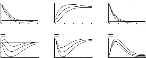
Figure 1 plots the impulse-response functions and the 10% error bands generated by Monte Carlo simulation, where we consider the full sample. The panels represent the response of investment to a one standard deviation shock in the other variables of the VAR. The impact on investment of a shock to GDP is positive, re‡ecting the co-movement that one typically …nds in real business cycles. Also, as predicted by the neoclassical model of investment, a shock in the cost of capital has a negative e¤ect on investment (of almost -1%) that lasts for 5 quarters. The investment shocks tend to persist for about 10 quarters, and reveal the strong persistence of investment growth. In what concerns the …nancial variables, the response of investment to a shock in the lending rate suggests that investment gradually falls after the shock and the trough of around -0.4% is reached after 5 quarters. In line with the Tobin’s Q approach, it can also be seen that a shock to the equity price has a positive and sizeable impact on investment (around 2% increase) which peaks after 3 quarters and lasts for about 12 quarters. As a result, the empirical …ndings seem to support the idea that capital markets play a role that is more in‡uential than monetary policy itself.

Summing up, the results are in accordance with Peltonen et al. (2009), as they highlight a strong role for "fundamental" factors, but also provide evidence of an important linkage to "…nancial factors" and to the capital markets.

Figure 1: Impulse-response functions: using the full sample.

The response of investment to a shock in credit is interesting: investment starts falling after the shock, the trough of about -1% is reached after 5 quarters, and then starts recovering. This result may be related with the fact that our approach does not allow us to disentangle between credit supply and credit demand shocks. As Bernanke and Blinder (1988) show, a positive credit demand shock is contractionary for GDP, lowers the money supply but also raises credit. As a result, a monetarist central bank would turn expansionary and would cut

8