3. Статья NIPE_WP_19_2009

the interest rates, therefore, boosting investment. A positive credit supply shock has, however, an expansionary e¤ect on GDP, and increases both credit and money supply. Consequently, the central bank would try to stabilize the economy by increasing the interest rates, which would have a negative e¤ect on investment.

The pattern of the response of investment to a shock in credit seems, therefore, to suggest that our approach is capturing the e¤ects of a credit demand shock, which would push up the interest rates and, consequently, have a negative impact on investment. In contrast, if the developments in credit markets were driven by the supply side, one should observe a fall in the interest rates following the shock to credit.

Figure 2 shows the response of lending rate to the shock to credit and con…rms our hypothesis: the lending rate increases after the shock, reaches a peak of about 60 basis points after 3 quarters and, then, starts gradually falling.

Figure 2: The response of lending rate to a shock to credit.

Response of LENDRATE to Shock in CREDIT

Table 1 presents the variance decompositions for our PVAR model, where we use the full sample. We look at the percent of variation in the row variable (20 quarters ahead) explained by column variable, accumulated over time. The results show that the GDP (a fundamental factor) and the equity price (which proxies the Tobin’s Q) explain a very important fraction of the investment variation 20 quarters ahead (respectively, 28.9% and 19.8%). In contrast, the cost of capital (another fundamental determinant of investment in the neoclassical model) and the …nancial factors (credit and the lending rate) play a secondary role, as they represent a small share of the variation of investment (respectively, 1.2%, 4.6% and 0.8%).

9

Table 1: Variance decompositions.

Note: Percent of variation in the row variable (20 quarters ahead) explained by column variable.

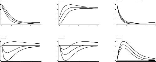
We now look at the response of investment to shocks to the di¤erent variables of the system by geographical area. Figure 3 plots the impulse-response functions and the 10% error bands generated by Monte Carlo simulation for emerging Asia. Figure 4 summarizes the information for Latin American markets. Figure 5 displays the results for emerging European economies.

The results are overall consistent with the …ndings for the full sample. However, one can still emphasize that: (i) investment in all geographical regions exhibit a strong co-movement with GDP; (ii) the cost of capital has a temporary and negative impact on investment, especially, in Latin America and emerging Europe; (iii) the negative e¤ect of lending rate on investment is more pronounced and signi…cant for emerging European markets, re‡ecting the fact that these economies tend to be bank-based;9 (iv) credit shocks have a negative and signi…cant e¤ect in Latin America; and (v) equity price shocks have a positive impact of similar magnitude for Asia and Latin America, but the e¤ects tend to be smaller for emerging Europe.

9 Edison and Slok (2003) also show that wealth e¤ects on consumption are typically larger in countries that are market-based (i.e., where the role of the …nancial market is prominent) than in countries that are bank-based (i.e., where the …nancial system is based on bank loans). Two explanations are o¤ered: (i) the share of …nancial assets in total wealth is larger for households and …rms in the market-based group; and (ii) households and …rms can borrow more easily against their assets in market-based economies due to deeper …nancial deregulation and wider …nancial instruments.

10

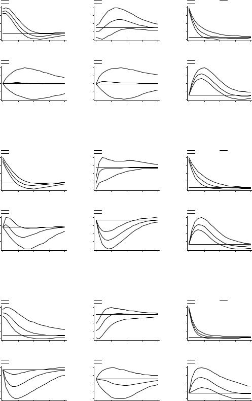
Figure 3: Impulse-response functions: sample of emerging Asian markets.

Figure 4: Impulse-response functions: sample of Latin America markets.

Figure 5: Impulse-response functions: sample of emerging European markets.

11

6Sensitivity analysis

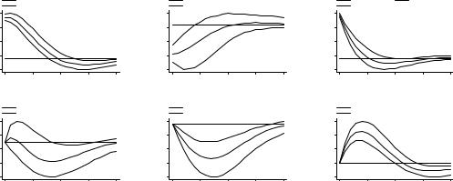
We start by looking at the impulse-response functions for di¤erent sub-samples. We consider two periods: 1990:1-1999:4 (Figure 6) and 2000:1-2008:3 (Figure 7). The major di¤erence between the two sub-samples lie on the response of investment to a shock to the equity price. In fact, the results suggest that the e¤ects are stronger in the period 1990:1-1999:4 (a peak of about 3% reached after 3 to 5 quarters which compares with roughly 1% in the period 2000:1-2008:3), re‡ecting the boom of stock markets in that period, which may have, therefore, contributed to amplify investment growth. While this may be supporting the Tobin’s Q approach, it is also in accordance with the …ndings of Caballero and Hammour (2002) who suggest that stock market bubbles may encourage real investment and with the work of Edison and Slok (2003) who argue that …rms have exploited part of the increase in stock market valuations in the nineties to rise their investment.

In addition, the results also show that: (i) the sensitivity of investment with respect to shocks to GDP was larger in the …rst sub-sample, probably, re‡ecting a stronger co-movement between the two macroeconomic aggregates and the instability associated to episodes of crises; (ii) investment has become less responsive to shocks in the cost of capital (iii) the negative response of investment to shocks in the lending rate is smaller in magnitude and shorter in duration in the period 2000:1-2008:3; and (iv) while a positive credit shock impacts negatively on investment in the …rst sub-sample, it seems to produce a positive (although) lagged response of investment in the second sub-sample. This piece of evidence is consistent with the idea that constraints in the access to credit were more important during the nineties, when, not surprisingly, credit demand shocks played an important role. In contrast, the period of 2000:1-2008:3 was characterized by an easier access to international capital markets, stronger …nancial linkages, deeper global imbalances and, in general, expansionary monetary policy. As a result, credit supply shocks seem to be more prominent in this period, thereby generating a positive e¤ect on investment.

Figure 6: Impulse-response functions: sub-sample period 1990:1-1999:4.

12

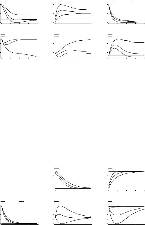
Figure 7: Impulse-response functions: sub-sample period 2000:1-2008:3.

We now drive the attention to the framework that focuses on the fundamental (or neoclassical) and the …nancial determinants of investment. In practice, we drop the equity price, EQ, from the set of variables of the PVAR model. This empirical exercise aims at analyzing whether the previous results are somewhat biased by the presence of a variable that is related with markets where trade takes place instantaneously. Moreover, it assesses whether the equity price is just capturing useful leading information about investment opportunities, in particular, and the economy, in general.

The results can be found in Figure 8 and clearly show that the previous conclusions do not change: (i) a shock to GDP has a positive impact on investment, re‡ecting the co-movement between the two macroeconomic aggregates; (ii) the cost of capital has a negative (although temporary) e¤ect on investment; and (iv) shocks to investment tend to be persistent; and (iv) a shock to credit has a negative e¤ect on investment that gradually dissipates as the shock erodes. Nevertheless, the response of investment to a shock in the lending rate becomes insigni…cant.

Figure 8: Impulse-response functions: without EQ.

13

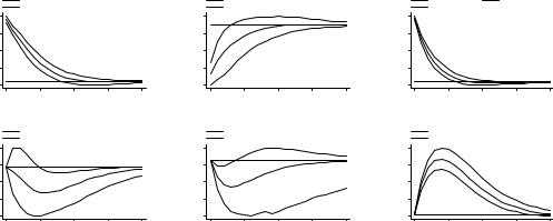
Figure 9 displays the impulse-response functions of the model where we replace CREDIT by MONEY . Bernanke and Blinder (1988) show that a creditist central bank reacts di¤erently to observable variables (for instance, income, money and credit) than a monetarist central bank. We, therefore, use MONEY (instead of CREDIT ) in our PVAR model. The results remain robust relative to the previous …ndings. Noticeably, the negative response of investment (that one observed for the credit shock) de facto disappears, as it becomes statistically not signi…cant after a few quarters in the case of the monetary aggregate. As a result, a shock to MONEY can be associated with an improvement of the liquidity conditions: by increasing the level of liquidity in the economy and reducing the number of liquidityconstrained companies, a shock to the monetary aggregate may actually induce an increase of private investment.

Finally, given that emerging markets have frequently been the stage for episodes of economic, …nancial and/or currency crises, we create two dummy variables, Di;tCRISIS and Di;tNO CRISIS, aimed at identifying them. We de…ne the dummy variable Di;tCRISIS as follows: it takes the value of 1 if either the change (year-on-year) of real GDP or real equity price index is more than two times the country-speci…c standard deviation of the variable; and 0, otherwise. In addition, the quarters before and after the peak of crisis are also marked with 1, and all other periods (normal periods) are marked with 0. By its turn, the dummy variable Di;tNO CRISIS takes the value of 1 in case of absence of episodes of crises and 0 otherwise. Then, we estimate a dummy variable augmented PVAR model of the form:

This robustness test checks whether the previous …ndings were biased because the episodes of crises were not appropriately controlled for. Figure 10 displays the impulse-response functions in the case of NO CRISIS scenario. The results support the robustness of the previous

14

…ndings and show that, in the absence of periods of extreme instability (that is, in "normal" periods), investment still responds in the same manner to shocks in the di¤erent variables of the system.

Figure 10: Impulse-response functions: absence of episodes of crises.

7Conclusion

This paper uses a Panel Vector Auto-Regressive (PVAR) approach to analyze the short-run dynamics of private investment to shocks to fundamental and …nancial factors in emerging market economies.

By relying on a panel of 31 emerging economies and quarterly frequency data for the period 1990:1-2008:3, we show that: (i) the persistence of investment shocks is large; (ii) there is a strong co-movement between investment and GDP; (iii) shocks to the equity price have a positive and sizeable impact on investment; (iv) unexpected variation in the cost of capital has a negative (although temporary) e¤ect on investment; (v) credit demand shocks seem to be particularly important. The robustness of these …ndings is also assessed against the exclusion of the equity price index and the presence of crises episodes.

The negative response of investment to the credit shock de facto disappears and becomes not statistically signi…cant after a few quarters when the measure of credit is replaced by a monetary aggregate. Therefore, by increasing the level of liquidity in the economy, a shock to the monetary aggregate may actually induce an increase of private investment.

In addition, we show that the e¤ects of equity price shocks are of similar magnitude in emerging Asia and Latin America, but unexpected variation in credit conditions has more pronounced e¤ects in Latin America. Moreover, shocks to the lending rate have a negative e¤ect in emerging European markets, a fact that can be explained by the higher reliance of the …nancial system on bank loans.

Finally, we show that the impact of the equity price on investment was stronger in the …rst half of the sample, that is, 1990:1-1999:4. It, therefore, suggests that the boom of stock markets may have ampli…ed investment growth in emerging markets and that stock market bubbles may have, indeed, encouraged real investment. This piece of evidence should be

15

carefully addressed as it poses important challenges to emerging markets, in particular, in the case of a downturn of …nancial markets.

References

[1]Abel, A, and O. Blanchard (1986). The present value of pro…ts and the cyclical movements in investment. Econometrica, 54(2), 249-273.

[2]Andersen, M., and R. Subbaraman (1996). Share prices and investment. Reserve Bank of Australia, Research Discussion Paper No. 9610.

[3]Arellano, M., and S. Bond (1991). Some tests of speci…cation for panel data: Monte Carlo evidence and an application to employment equations. Review of Economic Studies, 58(2), 277-297.

[4]Arellano, M., and O. Bover (1995). Another look at the instrumental variables estimation error component models. Journal of Econometrics, 68(1), 29-51.

[5]Aschauer, D. A.( 1989). Does public capital crowd out private capital? Journal of Monetary Economics, 24(2), 171-188.

[6]Assenmacher-Wesche, K., and S. Gerlach (2008a). Financial structure and the impact of monetary policy on asset prices. Goethe University of Franfkurt, Working Paper.

[7]Assenmacher-Wesche, K., and S. Gerlach (2008b). Monetary policy, asset prices and macroeconomic conditions: a panel-VAR study. Goethe University of Franfkurt, Working Paper.

[8]Auerbach, A. J. (1983). Taxation, corporate …nancial policy, and the cost of capital.

Journal of Economic Literature, 21(3), 905-940.

[9]Barro, R. (1990). The stock market and investment. Review of Financial Studies, 3(1), 115-131.

[10]Beaudry, P., and F. Portier (2006). Stock prices, news, and economic ‡uctuations. American Economic Review, 96(4), 1293-1307.

[11]Beck, T., G. Clarke, A. Gro¤, P. Keefer, and P. Walsh (2001). New tools in comparative political economy: the database of political institutions. The World Bank Economic Review, 15(1), 165-176.

[12]Beetsma, R., Giuliodori, M., and F. Klaassen (2006). Trade spill-overs of …scal policy in the European Union: a panel analysis. Economic Policy, 21(48), 639-687.

[13]Beetsma, R., Giuliodori, M., and F. Klaassen (2008). The e¤ects of public spending shocks on trade balances and budget de…cits in the European Union. Journal of the European Economic Association, 6(2-3), 414-423.

[14]Bernanke, B., and A. Blinder (1988). Credit, money, and aggregate demand. American Economic Review, 78(2), 435–439.

16

[15]Bernanke, B., and M. Gertler (1989). Agency costs, net worth, and business ‡uctuations.

American Economic Review, 79(1), 14–31.

[16]Blanchard, O. J., and D. Quah (1989). The dynamic e¤ects of aggregate demand and supply disturbances. American Economic Review, 79(4), 655-673.

[17]Blanchard, O., C. Rhee, and L. Summers (1993). The stock market, pro…t, and investment. The Quarterly Journal of Economics, 108(1), 115-136.

[18]Blejer, M., and M. Khan (1984). Government policy and private investment in developing countries. IMF Sta¤ Papers, 31(2), 379-403.

[19]Blundell, R., and S. Bond (1998). Initial conditions and moment restrictions in dynamic panel data models. Journal of Econometrics, 87(1), 115–143.

[20]Bond, S., and A. Malik (2007). Explaining cross-country variation in investment: the role of endowments, institutions and …nance. Oxford University, Working Paper.

[21]Borensztein, E. (1990). Debt overhang, credit rationing, and investment. Journal of Development Economics, 32(2), 315-335.

[22]Bosworth, B. (1975). The stock market and the economy. Brookings Papers on Economic Activity, 2, 257-290.

[23]Brainard W., and J. Tobin (1968). Pitfalls in …nancial model building, American Economic Review, 58(2), 99-122.

[24]Caballero, R., and M. L. Hammour (2002). Speculative growth, NBER Working Paper No. 9381.

[25]Calomiris, C., and R. Hubbard (1989). Price ‡exibility, credit availability, and economic ‡uctuations: evidence from the United States, 1894-1909. Quarterly Journal of Economics, 104(3), 429-452.

[26]Canova, F., and M. Ciccarelli (2006). Estimating multi-country VAR models, ECB Working Paper No. 603.

[27]Canova, F., and E. Pappa (2007). Price di¤erentials in monetary unions: the role of …scal shocks, Economic Journal, 117(520), 713-737.

[28]Chirinko, R. S. (1993), Business …xed investment spending: a critical survey of modeling strategies, empirical results, and policy implications. Journal of Economic Literature, 31(4), 1875-1911.

[29]Chirinko, R. S., and H. Schaller (1996). Bubbles, fundamentals, and investment: a multiple equation testing strategy. Journal of Monetary Economics, 38(1), 47-76.

[30]Chirinko, R. S., S. M. Fazzari, and A. P. Meyer (1999). How responsive is business capital to user cost? An exploration with micro data. Journal of Public Economics, 74(1), 53-80.

[31]Chirinko, R. S., S. M. Fazzari, and A. P. Meyer (2004). That elusive elasticity: a longpanel approach to estimating the capital-labor substitution elasticity. CESifo Working Paper No. 1240.

17

[32]Christiano, L., Eichenbaum, M., and C. L. Evans (1999). Monetary policy shocks: what have we learned and to what end?. in Taylor, J., and M. Woodford (eds.). Handbook of Macroeconomics, 1A. Amsterdam: Elsevier.

[33]Christiano, L., Eichenbaum, M., and C. L. Evans (2005). Nominal rigidities and the dynamic e¤ects of a shock to monetary policy. Journal of Political Economy, 113(1), 1-45.

[34]Cummins, J. G., K. A. Hassett, and R. G. Hubbard (1994). A reconsideration of investment behavior using tax reforms as natural experiments. Brookings Papers on Economic Activity, 25(2), 1–59.

[35]Dees, S., di Mauro, F., Pesaran, M. H., and V. Smith (2006). Exploring the international linkages of the euro area: a Global VAR analysis, Journal of Applied Econometrics, 22(1), 1-38.

[36]Demirguc-Kunt, A., and V. Maksimovic (1998). Law, …nance, and …rm growth. Journal of Finance, 8(6), 2107-2137.

[37]Devereux, M., M. J. Keen, and F. Schiantarelli (1994). Corporate tax asymmetries and investment: evidence from UK panel data. Journal of Public Economics, 53(3), 395-418.

[38]Doan, T., R. B. Litterman, and C. Sims (1984). Forecasting and conditional projection using realistic prior distributions. Econometric Reviews, 3(1), 1-100.

[39]Dornbusch, R., and A. Reynoso (1989). Financial factors in economic development, NBER Working Paper No. 2889.

[40]Edison, H., and T. Slok (2003). The impact from changes in stock market valuations on investment: new economy versus old economy. Applied Economics, 35(9), 1015-1023.

[41]Fazzari, S. M., Hubbard, R. G., and B. C. Petersen (1988). Financing constraints and corporate investment. Brookings Papers on Economic Activity, 19(1), 141-206.

[42]Fischer, S., and R. Merton (1984). Macroeconomics and …nance: the role of the stock market, Carnegie-Rochester Conference Series on Public Policy, 21(1), 57-108.

[43]Froot, K., S. Claessens, I. Diwan, and P. Krugman (1991). Market-based debt reduction for developing countries: principles and prospects. Washington, D.C.: World Bank (IBRD).

[44]Fry, M. (1980). Saving, investment, growth and the cost of …nancial repression. World Development, April 1980, 317-327.

[45]Gallegati, M., and L. Stanca (1999). The dynamic relation between …nancial positions and investment: evidence from company account data. Industrial and Corporate Change, 8(3), 551–572.

[46]Galeotti, M., and F. Schiantarelli (1994). Stock market volatility and investment: do only fundamentals matter? Economica 61(242), 147-65.

[47]Gavin, W., and A. Theodorou (2005). A common model approach to macroeconomics: using panel data to reduce sampling error. Journal of Forecasting, 24(3), 203-219.

18