

page 19
•These methods are quite well suited to matrix solutions
•Lets consider a simple problem,
Find Vo |
|
10Ω |
|
20Ω |
|
|
|
+ |
|
|
|
|
|
|
+ |
|
I1 |
|
I2 |
|
|||
|
|
|
Vo |
||||
|
|
|
|||||
30V |
|
|
|||||
|
40Ω |
|
|
40Ω |
|||
|
|
|
|
||||
- |
|
|
|
|
|
|
|
|
|
|
5Ω |
|
30Ω |
|
- |
|
|
|
|
|
|||
|
|
|
|
|
|
|
|
After adding the mesh currents (and directions) we may write equations,
∑
∑
VI1 |
= 0 = – 30 + 10I1 + 40( I1 – I2) + 5I1 |
|
|
30 = 55I1 – 40I2 |
(1) |
VI2 |
= 0 = 20I2 + 40I2 + 30I2 + 40( I2 – I1) |
|
|
0 = 40I1 – 130I2 |
(2) |
Solve the equation matrix for I2, (I will use Cramer’s Rule)
|
|
|
|
|
|
|
|
|
|
|
|
|
|
|
|
|
|
|
|
|
|
|
|
|
|
det |
|
55 |
30 |
|
|
|
|
|
|
|
|
||||
55 |
–40 |
30 |
|
|
|
|
|
|||||||||||||
|
|
|
40 |
0 |
|
|
|
|
|
|
55( 0) |
– 30( 40) |
|
|||||||
|
|
|
|
|
|
|
|
|
|
|
|
|
|
|
||||||
40 |
–130 |
0 |
|
I2 = --------------------------------- |
|
|
|
|
= |
------------------------------------------------------ |
= 0.216A |
|||||||||
|
|
|
|
|
|
|
|
|
|
|
|
|
|
|
|
|
55 |
( –130) |
– ( –40) ( 40) |
|
|
|
|
|
|
det |
|
55 |
|
–40 |
|
|
|
||||||||
|
|
|
|
|
|
|
|
|
|
|
|
|
||||||||
|
|
|
|
|
|
|
40 |
–130 |
|
|
|
|
|
|
||||||
|
|
|
|
|
|
|
|
|
|
|
|
|
|
|
|
|
|
|
|
|
Finally calculate the voltage across the 40 ohm resistor,
VO = 40I2 = 8.6V
3.1.4 More Advanced Applications

page 20
3.1.4.1 - Voltage Dividers
• The voltage divider is a very common and useful circuit configuration. Consider the circuit below, we add a current loop, and assume there is no current out at Vo,
|
|
|
|
|
|
|
|
|
|
R1 |
|
|
|
|
|
|
|
|
|
|
|
|
|
+ |
|
I |
|
|
|
|
|
|
|
|
|
|
|
|
|
|
|
|
|
|
|
|
|
|
|
|
|
|
|
|
|
|
|
|
|
|
|
|
|||
Vs |
|
|
|
|
|
|
|
|
|
|
|
|
|
|
|
|
|
|
|
||
- |
|
|
|
|
|
|
|
|
|
|
|
|
|
|
|
+ |
|
|
|||
|
|
|
|
|
|
|
|
|
|
|
|
|
|
|
|
|
|||||
|
|
|
|
|
|
|
|
|
|
|
|
|
|
|
|
|
|
|
|
||
|
|
|
|
|
|
|
|
|
|
R2 |
|
|
|
|
|
|
Vo |
|
|
||
|
|
|
|
|
|
|
|
|
|
|
|
|
|
|
|
|
|
|
|||
|
|
|
|
|
|
|
|
|
|
|
|
|
|
|
|
|
|
- |
|
|
|
|
|
|
|
|
|
|
|
|
|
|
|
|
|
|
|
|
|
|
|
|
|
|
|
|
|
|
|
|
|
|
|
|
|
||||||||||
First, sum the voltages about the loop, |
|
|
|
|
|
|
|
||||||||||||||
|
|
∑ |
|
V = – Vs + IR1 + IR2 |
= 0 |
|
|
|
|
|
I = |
Vs |
|||||||||
|
|
|
|
|
|
|
----------------- |
||||||||||||||
|
|
|
|
|
|
|
|
|
|
|
|
|
|
|
|
|
|
|
|
|
R1 + R2 |
Next, find the output voltage, based on the current, |
|
||||||||||||||||||||
|
|
|
|
|
|
|
|
|
|
|
|
|
|
|
|
|
|
|
|
|
|
|
|
V |
|
= IR |
|
= |
|
|
|
Vs |
R |
|
= |
V |
|
|
|
R2 |
|
|
|
|
|
|
|
----------------- |
|
------------------ |
|
||||||||||||||
|
|
|
o |
|
2 |
|
R |
1 |
+ R |
|
2 |
|
|
|
s |
R |
1 |
+ R |
|
||
|
|
|
|
|
|
|
|
2 |
|
|
|
|
|
|
|
|
2 |
|
|||
page 21
ASIDE: variable resistors are often used as voltage dividers. As the wiper travels along the resistor the output voltage changes.
Vs +
Vo
3.1.4.2 - The Wheatstone Bridge
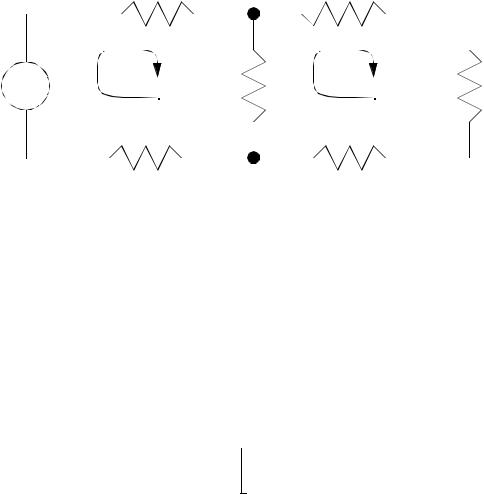
• The wheatstone bridge is a very common engineering tool for magnifying and measuring signals. In this circuit a supply voltage Vs is used to power the circuit. Resistors R1 and R2 are generally equal, Rx is a resistance to be measured, and R3 is a tuning resistor. An ammeter is shown in the center, and resistor R3 is varied until the current in the center Ig is zero.

page 22
|
|
|
|
|
|
|
|
|
|
|
|
|
|
|
|
R1 |
|
R2 |
|
|
|
|
|
|
|
|
|
|
|
|
|
+ |
|
|
|
|
|
|
|
|
|
|
|
|
|
|
|
|
|
Vs |
|
|
|
|
|
|
Ig |
||
|
|
|
|
|
|
||||
|
|
|
|
|
|
|
|
||
|
|
|
|
|
|
|
|
|
|
|
|
|
|
|
|
|
|
|
|
Rx
R3
For practice try to show the relationship below holds for a balanced bridge (ie, Ig=0),
Rx = |
R2R3 |
----------- |
|
|
R1 |
3.1.4.3 - Tee-To-Pi (Y to Delta) Conversion
•It is fairly common to use a model of a circuit. This model can then be transformed or modified as required.
•A very common model and conversion is the Tee to Pi conversion in electronics. A similar conversion is done for power circuits called delta to y.

page 23
a |
|
|
|
|
b |
a |
|
Rc |
|||
|
|
|
|
|
|
|
b |
||||
|
|
Rc |
|
|
|
|
|
|
|||
|
|
|
|
Ra |
|
|
Rb |
|
Ra |
||
|
Rb |
|
|
|
|||||||
c |
|
|
|
|
c |
c |
|
|
c |
||
|
|
|
|
|
|
||||||
|
|
|
|
|
|
|
|
|
|
||
|
|
Pi |
|
|
|
Delta |
|||||
|
a |
R1 |
|
R2 |
a |
|
|
b |
|||||
|
|
|
|
|
b |
|
|
|
|
|
|
|
|
|
|
|
|
|
|
|
|
R1 |
|
R2 |
|
|
|
|
|
|
|
|
|
|
|
|
|
|
|
||
|
|
|
R3 |
||||||||||
|
|
|
|
|
|
|
|
|
|
||||
c |
|
|
|
|
c |
|
|
R3 |
|
|
|
|
|
|
|
|
|
|
|
|
|
||||||
|
|
|
|
c |
|
|
c |
||||||
|
|
|
|
|
|
|
|
|
|||||
|
|
|
Tee |
|
|
|
|
|
|
|
|||
|
|
|
|
|
|
Y |
|||||||
|
|
|
|
|
|
|
|
|
|
||||
• We can find equivalent resistors considering that, |
|
|
|
|
|
|
|
||||||
page 24
Rac |
= |
1 |
= R1 |
+ R3 |
|
R |
|
( R |
|
+ R ) |
|
|
|
|
|
b |
c |
|
|
|
|||||||
|
1 |
+ |
1 |
|
|
|
|
a |
= |
R1 + R3 |
(1) |
||
|
----- |
+ Ra |
|
R------------------------------a + Rb + Rc |
|||||||||
|
Rb |
Rc |
|
|
|
|
|
||||||
Rab |
= |
1 |
= R1 |
+ R2 |
|
R |
|
( R |
|
+ R ) |
|
|
|
|
|
c |
a |
|
|
|
|||||||
|
1 |
+ |
1 |
|
|
|
|
b |
= |
R2 + R3 |
(2) |
||
|
----- |
+ Rb |
|
R------------------------------a + Rb + Rc |
|||||||||
|
Rc |
Ra |
|
|
|
|
|
||||||
Rbc |
= |
1 |
= R2 |
+ R3 |
|
R |
|
( R |
|
+ R ) |
|
|
|
|
|
a |
b |
|
|
|
|||||||
|
1 |
+ |
1 |
|
|
|
|
c |
= |
R2 + R3 |
(3) |
||
|
----- |
+ Rc |
|
R------------------------------a + Rb + Rc |
|||||||||
|
Ra |
Rb |
|
|
|
|
|
||||||
To find R1, (1)-(3)+(2) |
|
|
|
|
|
|
|
|
||||||||
|
Rb( Rc + Ra) – Ra( Rb + Rc) + Rc( Ra + Rb) |
|
||||||||||||||
|
----------------------------------------------------------------------------------------------------- |
|
|
|
|
|
Ra + Rb + Rc |
|
|
|
= R1 + R3 – R2 – R3 + R2 + R3 |
|||||
|
|
|
|
|
|
|
|
|
|
|
|
|||||
|
|
RbR |
c |
+ RbR |
a |
– RaR |
b |
– RaR |
c |
+ Rc R |
a |
+ RcR |
b = 2R1 |
|||
|
--------------------------------------------------------------------------------------------------------- |
|
|
|
|
|
|
|
||||||||
|
|
|
|
|
|
|
|
Ra + Rb + Rc |
|
|
|
|
||||
|
R1 |
= |
|
RbRc |
|
|
|
|
|
|
|
|
||||
|
R------------------------------a + Rb + Rc |
|
|
|
|
|
|
|
|
|||||||
|
|
|
|
|
|
|
|
|
|
|
|
|
||||
|
|
|
|
|
|
|
|
|
|
|
|
|
|
|
||
Likewise, |
|
|
|
|
|
|
|
|
|
|
|
|
|
|||
|
|
|
|
|
|
|
|
|
|
|
|
|
|
|
||
|
|
R2 |
= |
|
|
RaRc |
|
|
|
|
|
|
|
|
||
|
|
|
R------------------------------a |
+ Rb |
+ Rc |
|
|
|
|
|
|
|
|
|||
|
|
|
|
|
|
|
|
|
|
|
|
|
||||
|
|
R3 |
= |
|
|
RaRb |
|
|
|
|
|
|
|
|
||
|
|
|
R------------------------------a |
+ Rb |
+ Rc |
|
|
|
|
|
|
|
|
|||
|
|
|
|
|
|
|
|
|
|
|
|
|
||||
|
|
|
|
|
|
|
|
|
|
|
|
|
|
|
|
|
• To find the equivalents the other way,