

page 44
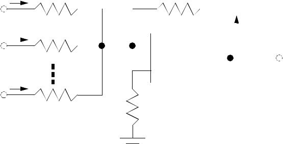
5.1.2.5 - Weighted Sums
• The following circuit can be used to add inputs. If dissimilar components are used the inputs can be weighted
page 45
I1
R1
V1 |
|
|
|
|
Rf |
|
|
|
If |
||||
|
|
|
|
|
|||||||||
|
|
|
|
|
|
|
|
|
|
|
|
||
|
I2 |
|
|
|
|
|
|
|
|||||
|
|
|
|
R2 |
|
|
|
|
|
|
|||
V2 |
|
|
|
|
|
|
|
Vo |
|||||
- |
|
|
|
|
|||||||||
|
|
|
|
|
|
|
|
|
|
|
|
|
|
|
|
|
|
|
|
|
|
|
|
|
|
|
|
+
In
Rn
Vn
We can recognize that the op-amp inputs are both kept at zero volts, and that there is not current into the non-inverting input, we can find,
V- |
= V+ = 0 |
|
|
|
|
|
|
|
|
|
|
|
|
|||||
I1 |
= |
V1 |
|
|
|
|
I2 = |
V2 |
|
|
|
|
In = |
Vn |
|
|
||
----- |
|
|
|
|
----- |
|
|
|
|
----- |
|
|
||||||
|
|
|
R1 |
|
|
|
|
|
|
R2 |
|
|
|
|
|
Rn |
|
|
If |
= |
Vo |
|
|
|
|
|
|
|
|
|
|
|
|
|
|
|
|
----- |
|
|
|
|
|
|
|
|
|
|
|
|
|
|
|
|||
|
|
|
Rf |
|
|
|
|
|
|
|
|
|
|
|
|
|
|
|
∑ |
|
I |
= |
I1 + I2 + In – If |
= 0 |
= |
V1 |
V2 |
+ |
Vn |
Vo |
|||||||
|
----- + ----- + … |
----- – ----- |
||||||||||||||||
|
|
|
|
|
|
|
|
|
|
|
|
|
R1 |
R2 |
|
Rn |
Rf |
|
|
|
|
|
|
|
|
|
|
|
|
|
|
|
|
|
|||
V |
|
= |
R |
V1 |
V2 |
+ … |
+ |
Vn |
|
|
|
|
|
|
||||
|
----- |
+ ----- |
----- |
|
|
|
|
|
|
|||||||||
|
|
o |
|
|
f R |
1 |
R |
2 |
|
|
R |
|
|
|
|
|
|
|
|
|
|
|
|
|
|
|
|
|
n |
|
|
|
|
|
|
||
5.1.2.6 - Difference Amplifier (Subtraction)
• We can construct an amplifier that subtracts one input from the other,

page 46
R2 |
|
|
Rf |
|
|
||
|
|
|
|
|
|||
V2 |
|
|
|
|
|
||
|
|
|
|
|
Vo |
||
|
|
|
- |
|
|
|
|
+ |
|
|
|
|
|||
|
|
|
|
||||
V1
R1
R3
Using the normal approach, we can see that both inputs are essentially voltage dividers,
V |
|
= V |
|
|
|
|
|
R3 |
|
|
|
|
|
|
|
|
|
----------------- |
|
|
|
|
|||||||
|
+ |
|
1 |
|
R |
1 |
+ R |
|
|
|
|
|||
|
|
|
|
|
|
|
|
|
3 |
|
|
|
|
|
V |
|
= ( V |
|
|
– V ) |
|
|
|
Rf |
+ V |
|
|||
|
|
|
---------------- |
|
||||||||||
|
- |
|
|
2 |
|
|
o |
|
R |
2 |
+ R |
|
o |
|
|
|
|
|
|
|
|
|
|
|
|
f |
|
|
|
Next, we can set the two inputs equal, and combine the equations,
|
V |
|
= V |
|
= V |
|
----------------- |
|
|
R3 |
|
= ( V |
|
– V ) ---------------- |
|
Rf |
|
+ V |
|
||||||||||||||
|
|
+ |
|
|
|
- |
|
|
|
|
1 R |
1 |
+ R |
|
|
|
|
|
|
2 |
|
|
o R |
2 |
+ R |
|
|
o |
|||||
|
|
|
|
|
|
|
|
|
|
|
|
|
|
3 |
|
|
|
|
|
|
|
|
|
|
|
|
|
|
f |
|
|
||
|
|
|
|
|
R2 + Rf – Rf |
|
|
|
|
|
R3 |
|
|
|
|
|
|
|
Rf |
|
|
|
|||||||||||
|
|
|
|
|
|
|
|
|
|
|
|
|
|
|
|
|
|
|
|
|
|
|
|
|
|
|
|||||||
|
Vo |
---------------------------- |
R |
2 |
+ R |
|
= V1 |
R------------------ |
1 |
|
+ R |
|
– V2 |
R---------------- |
2 |
+ R |
|
||||||||||||||||
|
|
|
|
|
|
|
|
|
|
f |
|
|
|
|
|
|
|
|
|
3 |
|
|
|
|
|
|
f |
|
|||||
|
V |
|
|
= |
V |
|
|
R3( R2 |
+ Rf) |
|
– V |
|
|
Rf |
|
|
|
|
|
|
|
|
|
||||||||||
|
|
|
|
----------------------------- |
|
( R |
|
|
|
|
----- |
|
|
|
|
|
|
|
|
|
|||||||||||||
|
|
|
o |
|
|
|
|
1 |
R |
2 |
1 |
+ R ) |
|
|
|
2 |
|
R |
|
|
|
|
|
|
|
|
|
|
|||||
|
|
|
|
|
|
|
|
|
|
|
|
3 |
|
|
|
|
|
|
|
2 |
|
|
|
|
|
|
|
|
|
||||
Note the result if all resistor values are equal, |
|
|
|
|
|
|
|
|
|
|
|||||||||||||||||||||||
|
Vo |
|
= V1 – V2 |
|
|
|
|
|
|
|
|
|
|
|
|
|
|
|
|
|
|
|
|
|
|
||||||||

page 47
5.1.2.7 - Op-Amp Voltage Follower
• At times we want to isolate a voltage source from an application, or add a high impedance. This can be done using a voltage follower,
- |
Vo |
VI |
+ |
|
|
|
|
We can develop some of the basic relationship for this circuit,
V+ = VI
V+ = V-
Vo = V-
Vo = VI
5.1.2.8 - Bridge Balancer
• Op-amps can be used for measuring the potential across bridges.