

page 57
6. AC CIRCUIT ANALYSIS
•There are a number of techniques used for analysing non-DC circuits.
•These techniques are,
-phasors - for single frequency, steady state systems
-laplace transforms - to find steady state as well as transient responses
-etc
6.1 PHASORS
•Phasors are used for the analysis of sinusoidal, steady state conditions.
•Sinusoidal means that if we measure the voltage (or current) at any point ‘i’ in the circuit it will have the general form,
Vi( t) = Vipeak sin ( ω it + φ i)
where, |
|
|
|
|
i |
= a node number |
|||
Vi( t) |
= |
the instantaneuous voltage at node i |
||
Vipeak |
= |
the peak voltage at node i |
||
ω |
i |
= |
the frequency of the sinusoid |
|
φ |
i |
= |
the phase shift |
|
•Steady state means that the transients have all stopped. This can be crudely though of as the circuit has ‘charged-up’ or ‘warmed-up’.
•Consider the example below,
page 58
+
R1 V1
-
-
Vs +
+
R2 V2
-
Considering that this is a simple voltage divider,
V |
|
= ( –V ) |
|
|
R2 |
|
----------------- |
||||
|
2 |
s |
R |
1 |
+ R |
|
|
|
|
2 |
|
If the supply voltage is sinusoidal we would find,
Vs |
|
= 95 sin ( 10t + 0.3) |
|
|
|
|
|
||
|
V |
|
= ( –95 sin ( 10t + 0.3) ) |
|
|
R2 |
|
||
|
------------------ |
||||||||
|
|
|
2 |
|
R |
|
+ R |
|
|
|
|
|
|
|
|
1 |
|
2 |
|
|
V |
|
|
= ( 95 sin ( 10t + 0.3 – π ) ) |
|
|
R2 |
|
|
|
|
----------------- |
|||||||
|
|
2 |
|
|
R + R |
||||
|
|
|
|
|
|
|
1 |
|
2 |
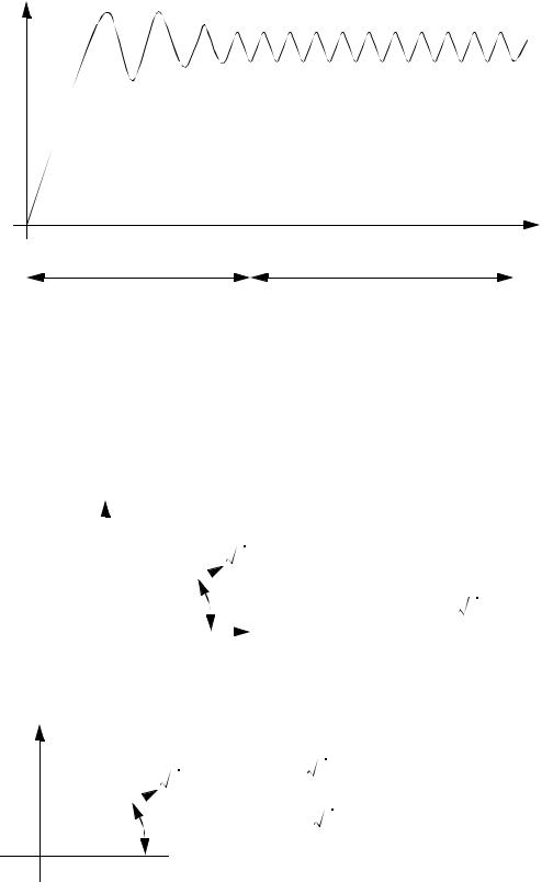
• Steady state is another important concept, it means that we are not concerned with the initial effects when we start a circuit (these effects are known as the transients). The typical causes of transient effects are inductors and capacitors.
page 59
V(t) |
t |
steady state + transients |
steady state |
• We typically deal with these problems using phasor analysis. In the example before we had a voltage represented in the time domain,
Vs = 95 sin ( 10t + 0.3)
We could also represent this in the polar domain using magnitude and phase shift. These Phase diagrams are only applicable for a single frequency. Note: the peak value is divided by the square root of 2 to convert it to an RMS value.
|
95 |
|
|
|
|
------V |
|
|
|
|
2 |
|
|
|
|
|
OR |
95 |
· |
|
|
Vs = ------V |
0.3rad |
|
|
0.3rad. |
2 |
|
|
|
|
|
|
|
|
|
|
|
|
|
|
|
|
|
Finally, we could represent the values in complex form,
imaginary
95 |
Vs |
= |
95 |
jφ |
} |
------V{ e |
|
||||
------V |
|
|
2 |
|
|
2 |
|
|
|
|
|
|
|
95 |
|
|
|
|
= |
|
|
||
|
------V{ cos ( 0.3rad) + j sin ( 0.3rad)} |
||||
0.3rad. |
|
|
2 |
|
|
|
|
|
|
|
|
 real
real

page 60
NOTE: When doing phasor analysis, it is assumed that all of the frequencies in the circuit are the same, and they only differ by a phase angle.
• Basically to do this type of analysis we represent all components voltages and currents in complex form, and then do calculations as normal.
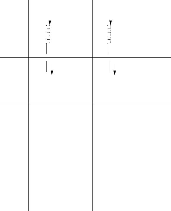
page 61
|
TIME DOMAIN |
PHASOR (FREQUENCY) DOMAIN |
|||||
|
|
|
|
|
|
|
|
RESISTOR |
|
I |
|
|
|
I |
|
|
|
|
|||||
|
|
|
|
|
|
||
+ |
|
|
+ |
|
|
|
|
|
|
|
|
|
|||
|
V |
|
|
V |
|
|
|
- |
R |
- |
Z = R |
||||
DC VOLTAGE |
|
|
I |
|
|
I |
|
|
|
|
|||
SOURCE |
Vs |
|
|
Vs |
|
|
|
|
|
|
|||
|
|
|
|
|
||
|
|
+ |
|
|
+ |
|
|
|
- |
|
|
- |
|
|
|
|
|
|
|
|
AC VOLTAGE |
|
I |
|
|
I |
|
|
|
|
|
|
|
|||
SOURCE |
|
Vs = A sin ( ω t + φ ) |
|
V |
|
A |
A |
|
|
|
|||||
|
|
|
|
||||
|
+ |
+ |
s |
= ------ cos φ |
+ j------ sin φ |
||
|
|
|
2 |
2 |
|||
|
- |
|
- |
|
|
||
|
|
|
|
|
|
||
|
|
|
|
|
|
|
|
CAPACITOR |
|
|
I |
|
|
|
I |
|
|
|
|
|
|
|
|
|
|||||
+ |
|
|
|
d |
+ |
|
|
Z = |
|
1 |
V |
|
|
|
C----V = I |
V |
|
|
--------- |
||
|
|
dt |
|
|
jω |
C |
||||
|
|
|
|
|
|
|||||
- |
|
|
|
|
- |
|
|
|
|
|
|
|
|
|
|
|
|
|
|
|
|
page 62
|
TIME DOMAIN |
PHASOR (FREQUENCY) DOMAIN |
|||||
|
|
|
|
|
|
|
|
INDUCTOR |
|
|
I |
|
|
I |
|
|
|
|
|
||||
|
|
|
|||||
+ |
|
|
d |
+ |
|
Z = jω L |
|
|
|
|
|||||
|
V |
|
V = L----I |
V |
|||
|
|
dt |
|
||||
- |
|
|
- |
|
|
||
|
|
|
|
|
|||
OHM’S LAW
+ |
|
|
I |
+ |
|
|
I |
|
|
|
|
||||
|
|
V = IR |
|
|
V = IZ |
||
V |
|
|
V |
|
|
||
|
|
|
|
|
|
||
- |
|
|
|
- |
|
|
|
|
|
|
|
|
|
|
|
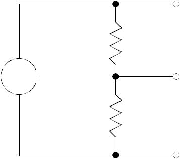
• Consider the simple example below,
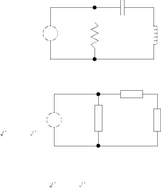
page 63
|
|
10µ F |
|
|
+ |
5Ω |
+ |
|
|
||
|
- |
5mH |
Vo |
|
|
- |
|
Vs |
= 5 sin ( 10000t + 0.5) |
|
|
|
|
We can redraw the diagram using impedances for each component,
|
|
|
|
Z2 |
= |
1 |
|
|
|
|
|
-------------------------------- |
|
||
|
|
|
|
|
|
j( 10000) 10–5 |
|
|
|
|
|
Z1=5Ω |
|
|
|
|
|
|
+ |
|
|
|
+ |
|
|
5 |
- |
Z3 |
= j( 10000) 0.005 |
Vo |
|
|
|
5 |
- |
||||
Vs |
= |
------ sin ( 0.5) + j------ cos ( 0.5) |
|
|
|
|
|
|
|
2 |
2 |
|
|
|
|
Then, as if the circuit is only made of resistors, we procede to use standard circuit analysis techniques,
|
|
|
|
|
|
|
|
|
|
|
|
|
|
|
Z3 |
|
|
5 |
|
5 |
|
|
j( 10000) 0.005 |
|
|
Vo = Vs Z----------------- |
2 |
+ Z |
= |
|
------2 |
sin ( 0.5) + j |
------2 |
cos ( 0.5) |
|
--------------------------------------------------------------------------1 |
|
|
|
3 |
|
|
|
|
|
-------------------------------- |
|
|
|||
|
|
|
|
|
|
|
|
|
|
j( 10000) 10–5 |
+ j( 10000) 0.005 |
|
|
Vo |
|
( j( 10000) 0.005) ( j( 10000) 10–5) |
|
= ( 3.11 + j1.70) |
--------------------------------------------------------------------------------------- |
|
||
|
|
|
1 + ( j( 10000) 0.005) ( j( 10000) 10–5) |
|
|
Vo |
= ( 3.11 + j1.70) |
|
5 |
|
= |
{ – 3.89 – j2.13} V = 4.43V –2.07rad |
|
|
1-----------– |
5 |
||||||
|
|
|
|
|
If we express the output voltage as a function of time we get,
Vo( t) = 4.43 sin ( 10000t – 2.07) V