

Горяйнов / Optimal Insurance Design Under a Value-at-Risk Framework
.pdfTHE GENEVA RISK AND INSURANCE REVIEW, 30: 161–179, 2005c 2005 The Geneva Association
Optimal Insurance Design Under a Value-at-Risk
Framework
CHING-PING WANG |
cpwang@isu.edu.tw |
Department of Finance, I-Shou University, No. 1, Section 1, Hsueh-Cheng Rd., Ta-Hsu Hsiang, |
|
Kaohsiung County, Taiwan |
|
DAVID SHYU |
dshyu@cm.nsysu.edu.tw |
Department of Finance, National Sun Yat-Sen University, No. 70, Lien-Hai Rd., Kaohsiung, Taiwan |
|
HUNG-HSI HUANG |
d86723002@ntu.edu.tw |
Department of Business Administration, Southern Taiwan University of Technology, No. 1, Nan-Tai Street, Yung-Kang, Taiwan
Received February 23, 2004; Revised December 16, 2004
Abstract
This study designs an optimal insurance policy form endogenously, assuming the objective of the insured is to maximize expected final wealth under the Value-at-Risk (VaR) constraint. The optimal insurance policy can be replicated using three options, including a long call option with a small strike price, a short call option with a large strike price, and a short cash-or-nothing call option. Additionally, this study also calculates the optimal insurance levels for these models when we restrict the indemnity to be one of three common forms: a deductible policy, an upper-limit policy, or a policy with proportional coinsurance.
Key words: value at risk, optimal insurance, deductible, policy limit, coinsurance
JEL Classification No.: G22
1. Introduction
This study focuses on deriving the optimal insurance policy form endogenously under a value-at-risk (VaR) framework, where VaR is defined as the worst expected loss over a given horizon at a given confidence level (Jorion [2001]). In this framework, the insured’s objective is to maximize expected final wealth, but has a VaR constraint that must be met. In addition to deriving the optimal insurance, this study also calculates the optimal insurance levels for three alternative insurances in which we restrict the indemnity to be one of three common forms: a deductible policy, an upper-limit policy, or a policy with proportional coinsurance.
At least three reasons exist why this study addresses the problem of the optimal insurance policy under a VaR framework. First, institutions frequently face different forms of risk,
Author to whom all correspondence should be addressed.
162 |
WANG, SHYU AND HUANG |
most of which can be insured, and VaR has been adopted by institutions around the world as a risk management tool.1 It is natural for institutions facing different forms of risk to purchase risk reducing insurance. For example, insurance policies now can be purchased to protect against losses such as human error, loss of staff, interruption of business, trading losses, technology failure, and so on. Second, every individual always faces the risk of uncertain future wealth and income. Like institutions, individuals can adopt VaR for risk management. Naturally, individuals can purchase insurance to control VaR. Third, VaR has progressively been adopted as the asset allocation constraint, for example, Campbell et al. [2001] and Basak and Shapiro [2001].2 Additionally, given a fixed confidence level, although bankers are frequently asked to calculate their VaR in order to determine their regulatory capital, however, bankers can also retain the current capital level and adjust their asset allocation, or can simply purchase insurance to meet their VaR criteria. Restated, bankers can meet both the given regulatory confidence level and VaR by purchasing insurance.
Various investigations have examined optimal insurance policy design. These investigations can be divided into two frameworks, with and without using expected utility. Under the expected utility framework, Arrow [1974], and Raviv [1979] derived the optimal policy form endogenously. Their studies assumed nonnegative indemnity and no moral hazard, but subsequent studies relaxed these assumptions. Huberman, Mayers, and Smith [1983] focused on two insurance policies, upper limits on coverage and deductibles, and incorporated moral hazard into their analysis. Next, Gollier [1987] relaxed the constraint that insurance payments are always nonnegative to analyze optimal insurance contracts. Under the non-expected utility framework, Doherty and Eeckhoudt [1995] adopted Yaari’s Dual Theory to derive the optimal insurance. Since expected utility is linear in probability but nonlinear in wealth, and since Yarri’s Dual Theory is linear in wealth but nonlinear in probability, Yaari’s Dual Theory generally obtains better results than expected utility theory. Next, using the framework of second-degree stochastic dominance, Gollier and Schlesinger [1996] provided a new proof for the optimality of deductible insurance, and Schlesinger [1997] examined insurance policy goodness.
Similar to most previous research, this study endogenously derives the optimal insurance policy form. However, unlike previous research, this study designs an optimal insurance under a VaR framework. Like Doherty and Schlesinger [1983a], Doherty and Eeckhoudt [1995], Li and Liu [2003], and Gollier [2003], this study assumes the insurance loading to be proportional to expected indemnity. The main contents of this study include the following: First, this study respectively derives the optimal insurance and the three alternative insurances without making any assumption regarding the probability density function of the risk. Second, to obtain more explicit indemnity schedules for all these insurance forms, this study further assumes that risk is uniformly distributed and lognormally distributed.
Section 2 derives the optimal insurance and alternative insurances under a VaR constraint. Sections 3 and 4 then present the optimal insurance and alternative insurances under the uniform and lognormal distributions, respectively. Finally, Section 5 presents conclusions.
OPTIMAL INSURANCE DESIGN |
163 |
2.The model
2.1.Assumptions
An insured has an initial wealth, W0, and faces a risk of loss, X , which is a non-negative continuous random variable with probability density function, f (x ) and cumulative distribution function, F (x ). An insurance policy can reduce this risk. The insurance policy costs a premium, P , and pays an indemnity schedule, I (x ), 0 ≤ I (x ) ≤ x for all x . Assume the insurer
is risk neutral and the premium accordingly has the form P = |
¯ |
¯ |
(1 + λ)I , where I and λ |
||
denote the expected indemnity payment and percentage loading, respectively. That is, the
¯
insurance cost is proportional to the expected indemnity payment and the loading fee is λ I . Consequently, the insured’s final wealth is W = W0 − P − X + I (X ) and expected final
¯ |
− P − x¯ |
¯ |
wealth is W = W0 |
+ I , where x¯ denotes the expected loss. |
This study assumes that the objective of the insured is to choose I (x ) to maximize the expected final wealth under the VaR constraint, where VaR is the worst expected loss over a given horizon at a given confidence level. Mathematically, the VaR constraint means
{ ≥ ¯ − } = − ≡ − = =
Pr W W v 1 α, where v VaR, 1 α the confidence level, and α the significance level.
2.2.Optimal insurance policy design
This subsection designs the optimal insurance that is Pareto-efficient, i.e. first-best optimal.3 The optimal insurance form with the indemnity schedule, I (x ), must sufficiently satisfy the insured’s objective and meet the premium request of the insurer. According to the previous subsection, the optimal I (x ) can be obtained as follows:
Maximize |
¯ |
¯ |
¯ |
|
|
|
(1) |
I (x ) |
W = W0 − P − x + I |
|
|
|
|||
Subject to |
¯ |
− v} ≥ 1 − α |
and |
¯ |
|
|
|
Pr {W ≥ W |
P = (1 + λ)I |
|
|
||||
|
¯ |
|
|
|
¯ |
|
− α |
Using equalities P = (1 + λ)I and W |
= W0 − P − X + I (X ), Pr {W ≥ W − v} ≥ 1 |
||||||
can be rewritten as |
|
|
|
|
|
|
|
|
|
¯ |
− α. |
|
|
|
(2) |
Pr{X − I (X ) ≤ v + x¯ − I } ≥ 1 |
|
|
|
||||
|
¯ |
|
|
¯ |
¯ |
, x¯ , and λ |
|
Substituting P = (1 + λ)I into eqaution (1) yields W = W0 − x¯ − λ I . Since W0 |
|||||||
do not depend on I (x ), eqaution (1) means to minimize the indemnity to reduce the loading fee. Accordingly, the optimality problem can be restated as follows.
Minimize |
¯ |
(3) |
I |
||
I (x ) |
|
|
Subject to equation (2) |
|
|
¯ |
|
¯ |
Minimizing I is equivalent to maximizing x¯ |
− I , since x¯ does not depend on I (x ). Con- |
|
sequently, the insured sets I (x ) to minimize loading fee. In fact, x − I (x ) represents the
164 WANG, SHYU AND HUANG
− ¯
retention of the loss, and thus x¯ I represents the expected retention. The constraint indicates
≡ + − ¯ the probability that the retention does not exceed the particular critical value, xˆ v x¯ I ,
at least equals the confidence level (1 − α).
Since equation (3) is difficult to solve directly, like Raviv [1979] and Gollier and Schlesinger [1996], we divide the optimality problem into two sub-problems. First, the premium P is assumed fixed and the form of the optimal insurance coverage is found as a
= + ¯
function of P . Second, the optimal P is chosen. Since P (1 λ) I , the fixed value of P
¯
is equivalent to fixed I .
¯ |
|
|
Considering a fixed value of I , the first sub-problem is to choose I (x ), which must satisfy |
||
¯ |
|
¯ |
the restriction of E [I (X )] = I and minimize the probability Pr {X − I (X ) > v + x¯ − I }. |
||
|
¯ |
= 0 |
To save the loading fee, we start considering no indemnity paid yet. That is, when I |
||
and then the corresponding indemnity schedule I (x ) ≡ |
¯ |
|
0 for all x . Substituting I = 0 and |
||
I (x ) ≡ 0 into equation (2), the constraint is changed to |
|
|
Pr {X ≤ v + x¯ } ≥ 1 − α |
|
(4) |
Accordingly, we obtain |
|
|
If Pr {X ≤ v + x¯ } ≥ 1 − α, then I (x ) ≡ 0 |
for all x . |
(5) |
This study starts to consider another case that does not satisfy equation (4), restated, the
¯
insured requires insurance and thus I > 0. Additionally, the constraint of equation (2) must be binding for optimality, since X has a continuous probability distribution. Accordingly, equation (3) can be rewritten as follows.
Minimize |
¯ |
|
|
|
(6) |
I |
|
|
|
||
I (x ) |
|
|
|
|
|
Subject to |
¯ |
} = 1 |
− α |
|
(7) |
Pr{X − I (X ) ≤ v + x¯ − I |
|
||||
|
|
|
¯ |
|
¯ |
Equation (7) is equivalent to Pr {X − I (X ) > v + x¯ − I |
} = α. Fixing a value of I > 0, |
||||
|
|
|
|
¯ |
}. For losses |
I (x ) must be chosen to minimize the probability Pr {X − I (X ) > v + x¯ − I |
|||||
|
¯ |
such that x > v + x¯ −4I , an indemnity can be paid to bring this to an equality, that is, |
|
¯ |
¯ |
I (x ) = x − (v + x¯ − I ). |
However, this might violate the restriction that E [I (X )] = I . To |
|
¯ |
save loading fees, the insured sub-interval is selected on the smaller part of x > v + x¯ − I . |
|
¯ |
A, where A is a particular critical |
The insured sub-interval is assumed to be v + x¯ − I < x < |
|
value. Since X is continuous, A is unique. In sum, in the case where Pr {X > v + x¯ } > α, the optimal indemnity schedule I (x ) is summarized as follows.
0 |
x ≤ xˆ |
|
|
If Pr {X > v + x¯ } > α, then I (x ) = x − xˆ |
xˆ |
< x < A |
(8) |
0 |
x |
≥ A |
|
¯ |
¯ |
¯ |
Since Pr {X − I (X ) > v + x¯ − I |
} is increasing in I . If we now increase (decrease) I , |
|
the minimum probability will fall (rise). Consequently, the second sub-problem is to adjust

OPTIMAL INSURANCE DESIGN |
165 |
¯
I such that the probability equals the value α. From equation (8), we can further obtain that
|
|
¯ |
|
|
≥ A} = 1 − F (A) = α |
(9) |
|
Pr {X − I (X ) > v + x¯ − I } = Pr {X |
|||||||
¯ |
= |
F −1(1 |
− |
|
· |
) denotes the inverse function of F . |
|
Equation (9) implies A |
|
|
α), where F −1( |
||||
Finally, I must be adjusted to satisfy the following equation: |
|
||||||
¯ |
A |
|
|
|
|
¯ |
|
|
(x − xˆ ) f (x ) d x , |
|
|
||||
I = E [I (X )] = |
xˆ |
xˆ ≡ v + x¯ − I . |
(10) |
||||
Actually, the condition Pr {X > v + x¯ } > α is equivalent to A > v + x¯ , since A = F −1(1 − α). Combining this with equations (5), (8), (9), and (10), the optimal indemnity
schedule is summarized as follows: |
|
|
|
I (x | A ≤ v + x¯ ) ≡ 0 |
for all x, |
(11) |
|
and |
|
|
|
0 |
x ≤ xˆ |
|
|
I (x | A > v + x¯ ) = |
x − xˆ |
xˆ < x < A. |
(12) |
0 |
x ≥ A |
|
|
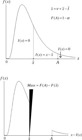
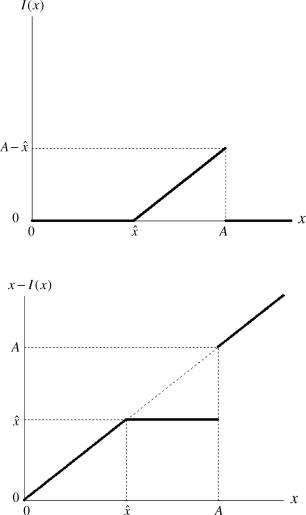
Additionally, the optimal indemnity schedule is listed in Table 1. Moreover, figure 1 indicates the probability density function of loss and shows the optimal indemnity schedule. To analyze the retained loss, this study draws the probability density function of retention (x − I (x )) in figure 2. Especially, the retained loss has a probability mass (= F (A) − F (xˆ )) at xˆ . Figures 3 and 4 respectively illustrate the relations of indemnity and retention versus loss.
Interestingly, the optimal indemnity schedule can be decomposed as three options. From equation (12), we obtain
I (x ) = Max {x − xˆ , 0} − Max {x − A, 0} − (A − xˆ ) × 1x ≥ A , |
(13) |
where 1x ≥ A , an index function, equals 1 if x underlying asset and taking the same maturity
≥ A and otherwise equals 0. Using x as the as the insurance policy, Max {x − xˆ , 0} and
Table 1. Optimal indemnity schedule.
Case |
A ≤ v + x¯ |
|
A > v + x¯ |
|
x interval |
x |
0 < x < xˆ |
xˆ < x < A |
A < x |
I (x ) |
I (x ) = 0 |
I (x ) = 0 |
I (x ) = x − xˆ |
I (x ) = 0 |
x − I (x ) |
x |
x |
xˆ |
x |
166 |
WANG, SHYU AND HUANG |
Figure 1. Probability density function of loss and optimal indemnity schedule.
Figure 2. Probability density function of retention.
Max {x − A, 0} are the call options with strike prices xˆ and A, respectively. By definition, a cash-or-nothing call option pays off nothing if the asset price ends up below the strike price at maturity, and pays a fixed amount if it ends up above the strike price (Hull [2003] p. 441). Taking A as the strike price and A − xˆ as the fixed amount, then (A − xˆ ) × 1x ≥ A is exactly equivalent to the payoff of a cash-or-nothing call option. In short, the optimal indemnity schedule is the same as a long call option with a small strike price, a short call option with a large strike price, and a short cash-or-nothing call option.
From equations (9) and (10), the main comparative static results can be derived as below, with the proofs being presented in Appendixes 1 and 2, respectively.
2 |
¯ |
/∂ ν |
2 |
> 0 |
¯ |
and |
2 |
¯ |
/∂ α |
2 |
> 0 |
¯ |
if A > xˆ . |
(14) |
∂ |
I |
|
> ∂ I /∂ ν |
∂ |
I |
|
> ∂ I /∂ α |
OPTIMAL INSURANCE DESIGN |
167 |
Figure 3. Indemnity versus Loss.
Figure 4. Retention versus Loss.
Assuming insurance is required (A > xˆ ),
demnity is decreasing and convex in ν and α.
¯ = − and concave in ν and α, since W W0 x¯
then based on equation (14), the expected inAccordingly, the expected wealth is increasing
−¯
λI . That is,
¯ |
2 ¯ |
2 |
and |
¯ |
2 ¯ |
2 |
if A > xˆ . |
(15) |
∂ W /∂ ν > 0 > ∂ |
W /∂ ν |
|
∂ W /∂ α > 0 > ∂ |
W /∂ α |
|
168 |
WANG, SHYU AND HUANG |
2.3.Alternative insurances
Case 1: Proportional coinsurance policy. Assume the indemnity schedule is limited to coinsurance provision, I (x ) = θ x , where θ denotes the coinsurance proportion. Accordingly, the optimality problem (equation (3)) is revised as follows.
Minimize |
¯ |
¯ |
|
|
|
|
|
|
|
(16) |
θ |
I = θ x |
|
|
|
¯ |
|
|
|
||
Subject to |
|
|
|
|
|
− α |
|
(17) |
||
Pr {X − θ X ≤ v + x¯ − I } ≥ 1 |
|
|||||||||
From equation (17), we obtain θ |
≥ |
1 |
− |
v/[F −1(1 |
− |
α) |
− |
x¯ ]. Substituting this fact into |
||
|
|
|
|
|||||||
equation (16) obtains |
|
|
|
|
|
|
|
|
|
|
θ = 1 − v/[F −1(1 − α) − x¯ ], |
|
|
|
|
|
|
(18) |
|||
I¯ = θ x¯ = {1 − v/[F −1(1 − α) − x¯ ]} x¯ . |
|
|
|
(19) |
||||||
¯
Equation (19) implies that the expected indemnity I is decreasing and liner in v.
Case 2: Deductible policy. Assume the indemnity schedule is limited to deductible clause, I (x ) = Max{x − D, 0}, where D represents the deductible. Accordingly, the optimality problem (equation (3)) is revised as follows.
Minimize |
¯ |
= |
∞ |
(x − D) f (x ) d x |
|
|
(20) |
|
|
|
|||||
D |
I |
D |
|
|
|||
Subject to |
|
|
|
¯ |
} ≥ 1 |
− α |
(21) |
Pr { Min {X, D} ≤ v + x¯ − I |
|||||||
Given Pr {X ≤ v + x¯ } ≥ 1 − α, from equation (5), the insured need not purchase insurance, i.e. I (x ) ≡ 0 or D ≥ Max {x }. Meanwhile, given Pr {X ≤ v + x¯ } < 1 − α, the
|
¯ |
insured should purchase insurance, that is, D < Max {x }. If the deductible D > v + x¯ − I , |
|
then equation (21) can be modified as follows. |
|
¯ |
(22) |
Pr {X ≤ v + x¯ − I } ≥ 1 − α. |
|
However, equation (22) clearly deviates the condition that Pr {X ≤ v + x¯ } < 1 − α.
¯ |
|
|
Therefore, D ≤ v + x¯ − I in the case that insured need purchase insurance. Taking the |
||
¯ |
¯ |
¯ |
constraint D ≤ v + x¯ − I into equation (20), D = v + x¯ |
− I since I is decreasing in D. |
|
In sum, the optimal deductible schedule can be arranged as follows. |
|
|
D ≥ Max{x } if Pr{X ≤ v + x¯ } ≥ 1 − α |
|
(23) |
OPTIMAL INSURANCE DESIGN |
|
169 |
||
and |
|
|
|
|
|
|
¯ |
|
|
D = v + x¯ − I |
|
|
||
I¯ = |
∞ |
(x − D) f (x ) d x |
if Pr{X ≤ v + x¯ } < 1 − α. |
(24) |
D |
||||
¯
Appendix 3 shows that the expected indemnity I is decreasing and convex in v.
Case 3: Upper-limit policy. Assume the indemnity schedule is limited to I (x ) = Min{x , M }, where M is the upper-limit. Accordingly, the optimality problem (equation (3)) is revised as follows.
Minimize |
¯ |
|
|
M |
∞ |
|
|
|
|
= |
|
x f (x ) d x + |
|
M f (x ) d x |
|
(25) |
|||
M |
I |
0 |
M |
|
|||||
Subject to |
|
|
|
|
|
¯ |
} ≥ 1 |
− α |
(26) |
Pr { Max{X, M } ≤ v + x¯ + M − I |
|||||||||
In the case where Pr {X ≤ v + x¯ } ≥ 1 − α, from equation (5), the insured need not purchase
insurance; that is, I (x ) ≡ 0 or M = 0. Meanwhile, when Pr {X ≤ v + x¯ } < 1 − α, the |
||||||||||||
|
|
|
|
|
|
|
|
|
|
|
|
¯ |
insured should purchase insurance; that is, M > 0. Since the inequality M < v + x¯ + M − I |
||||||||||||
always holds, equation (26) can be modified to |
|
|
|
|||||||||
|
|
¯ |
} ≥ 1 |
− α. |
|
|
|
|
|
(27) |
||
Pr {X ≤ v + x¯ + M − I |
|
|
|
|
|
|||||||
From equations (25) and (27), |
|
|
|
|
|
|
|
|
|
|
||
M |
|
|
|
|
|
|
|
|
F −1(1 |
|
|
|
x f (x ) d x |
− |
MF(M ) |
= |
v |
+ |
x¯ |
− |
− |
α), |
(28) |
||
0 |
|
|
|
|
|
|
|
|||||
and |
|
|
|
|
|
|
|
|
|
|
|
|
I¯ = v + x¯ + M − F −1(1 − α). |
|
|
|
|
|
|
(29) |
|||||
¯
Appendix 4 shows that the expected indemnity I is decreasing and concave in v.
3. Insurance policy under uniform distribution
Assume X obeys the uniform distribution, with probability density function
fU (x ) = 1/ h, 0 ≤ x ≤ h. |
(30) |
Accordingly, the cumulative distribution function
FU (x ) = x / h, 0 ≤ x ≤ h, |
(31) |

170 |
WANG, SHYU AND HUANG |
and the expected value |
|
x¯ = h/2.
For convenience, Uab is defined and calculated as follows.
U b |
≡ |
|
b x f |
|
(x ) d x |
= |
b x |
d x |
= |
b2 |
− a2 |
. |
|
|
U |
|
|
|
|||||||||
|
a h |
|
|
||||||||||
a |
a |
|
|
|
|
2h |
|||||||
From equations (5), (31) and (32), the condition that the loss requires insurance is
ν < (0.5 − α) h
For convenience, this Section assumes that equation (34) holds.
3.1.Optimal insurance
Combining equations (9) and (31) obtains
(32)
(33)
(34)
A |
F −1 |
(1 |
− |
α) |
= |
(1 |
− |
α)h. |
|
|
|
|
|
|
(35) |
|||||||
|
|
= U |
|
|
|
|
|
|
|
|
|
|
|
|
|
|
|
|||||
From equations (10), (30), (31), and (33), |
|
|
|
|
|
|
|
|||||||||||||||
|
|
A |
|
|
|
|
|
|
|
|
|
|
A |
|
|
|
|
|
¯ |
|
||
|
|
|
|
|
|
|
|
|
|
|
|
|
|
|
|
|
|
|
||||
|
xˆ |
(x − xˆ ) fU (x ) d x = Uxˆ − xˆ [FU (A) − FU (xˆ )] = I . |
(36) |
|||||||||||||||||||
|
|
|
|
|
|
|
|
|
|
¯ |
|
|
¯ |
|
|
|
|
|
|
|
||
Substituting xˆ = v + x¯ − I = v + h/2 − I and equation (35) into equation (36) yields |
||||||||||||||||||||||
|
(1 − α)2h2 − xˆ 2 |
|
|
xˆ |
|
(1 − α)h − xˆ |
|
v |
|
h |
|
xˆ . |
(37) |
|||||||||
|
|
|
− |
|
h |
= |
+ 2 |
− |
||||||||||||||
|
|
2h |
|
|
|
|
|
|
|
|
|
|
|
|
||||||||
Solving above equation obtains |
|
|
|
|
|
|
|
|
|
|
||||||||||||
xˆ = −α h + |
|
|
|
|
|
|
|
|
|
|
|
|
|
|||||||||
|
|
2 h (v + α h). |
|
|
|
|
|
|
(38) |
|||||||||||||
|
|
|
|
|
|
|
|
|
|
|
|
|
¯ |
|
|
|
|
|
|
|
|
|
Moreover, substituting xˆ = v + h/2 − I into equation (38) yields |
|
|||||||||||||||||||||
¯ |
|
|
|
|
|
|
|
|
|
|
|
|
|
|
|
|
|
|
|
|
|
|
|
|
|
+ α h − |
|
2 h (v + α h). |
|
|
|
|
|
|
(39) |
||||||||||
I = v + h/2 |
|
|
|
|
|
|
|
|||||||||||||||