

|
|
|
|
|
PROBE POOLING IN |
S. POMBE |
MAPPING |
305 |
ing to increase the throughput |
of experiments even further. However, the most efficient |
|
|
|
||||
ways to do this have not yet been worked out. |
|
|
|
|
|
|||
A caveat for all pooling approaches concerns the threshold between background noise |
|
|
|
|||||
or cross-hybridization and true positive hybridization signals. Theoretical, noise-free |
|
|
||||||
strategies are not likely to be viable with real biological |
samples. Instead of striving |
for |
|
|
||||
the most ambitious and efficient possible pooling strategy, it is prudent to use a more |
|
|
||||||
overdetermined approach and sacrifice a bit of efficiency for a margin of safety. It is im- |
|
|
|
|||||
portant to keep in mind that a pooling approach does not need to be perfect. Once poten- |
|
|
|
|||||
tial clones of interest are found or mapped, additional experiments can always be done to |
|
|
|
|||||
confirm their location. The key idea is to |
get the map approximately right with a mini- |
|
|
|
||||
mum number of experiments. Then the actual work involved in confirming the pooling is |
|
|
|
|||||
finite and can be done regionally by groups interested in particular locales. |
|
|
|
|||||
PROBE POOLING |
IN |
S. |
POMBE |
MAPPING |
|
|
|
|
An example of the power of pooling is illustrated by results obtained in ordering a cosmid |
|
|
|
|||||
library |
of the |
yeast |
S. pombe. |
This organism was chosen for a model mapping project |
|
|
||
because a low-resolution restriction map was already available and because of the interest |
|
|
|
|||||
in this organism as a potential target for genomic sequencing. An arrayed cosmid library |
|
|
|
|||||
was available. This was first screened by hybridization with each of the three |
|
S. pombe |
|
|||||
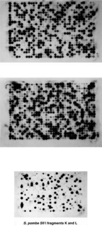
chromosomes purified by PFG. Typical results are shown in Figure 9.14. It is readily |
|
|
||||||
apparent that most cosmids fall clearly |
on one chromosome by their hybridization. |
|
|
|
||||
However there are significant variations in the amount of DNA present in each spot of the |
|
|
|
|||||
array. Thus a considerable amount of numerical manipulation of the data is required to |
|
|
|
|||||
correct for DNA sample variation, and for differences in the signals seen in successive |
|
|
||||||
hybridizations. When this is done, it is possible to assign, uniquely, more than 85% of the |
|
|
||||||
clones to a single chromosome based on only three hybridizations. |
|
|
|
|||||
The next step is to make a regional assignment of the clones. Here purified restriction |
|
|
||||||
fragments are labeled and used as hybridization probes with the cosmid array. An exam- |
|
|
|
|||||
ple is shown in Figure 9.15. Note that it is inefficient to use only a single restriction frag- |
|
|
||||||
ment at a time. For example, once one knows the chromosomal location of the cosmids, |
|
|
|
|||||
one can mix restriction fragments from different chromosomes and use them simultane- |
|
|
|
|||||
ously with little chance of introducing errors. After a small number of such experiments, |
|
|
|
|||||
one has most of the cosmids assigned to a well-defined region. |
|
|
|
|
||||
To fingerprint the cosmid array further, and begin to link up cosmid contigs, arbitrary |
|
|
|
|||||
mixtures of single-copy DNA probes were |
used. These were generated by the method |
|
|
|
||||
shown in Figure 9.16. A FIGE separation of a total restriction enzyme digest of |
|
S. pombe |
|
|||||
genomic DNA was sliced into fractions. Because of the very high resolution of FIGE in |
|
|
||||||
the size range of interest, these slices should essentially contain nonoverlapping DNA se- |
|
|
|
|||||
quences. Each slice was then used as a hybridization probe. As an additional fingerprint- |
|
|
|
|||||
ing tool, mixtures of any available |
S. pombe |
cloned single-copy sequences were made and |
|
|
||||
used as probes. For all of these data to be analyzed, it is essential to consider the quantita- |
|
|
||||||
tive hybridization signal, and correct it |
both for background and for differences in the |
|
|
|||||
amount of DNA in each clone, the day-to-day variations in labeling, and overall hy- |
|
|
||||||
bridization efficiency. |
|
|
|
|
|
|
||
The |
hybridization profile of |
each of the |
cosmid clones with the various probes used is |
|
|
|
||
an indication of where the clone is located. A likelihood analysis was developed to match
306 ENHANCED METHODS FOR PHYSICAL MAPPING
Figure 9.14 |
Hybridization of a cosmid array of |
S. pombe |
clones with intact |
S. pombe |
chromo- |
|
somes I ( |
a ) and II ( |
b ). |
|
|
|
|
Figure 9.15 |
Hybridization of the same cosmid array shown in Figure 9.14 with two large restric- |
||
tion fragments purified from the |
S. pombe |
genome. |
|
PROBE POOLING IN |
S. POMBE |
MAPPING |
307 |
high resolution separation of small restriction fragments by FIGE
purification of probe pools from gel slices
hybridization of probe pools to cosmid filter
gel
filter with cosmid DNA
Figure 9.16 Preparation of nonoverlapping pools of probes by high-resolution FIGE separation of
restriction enzyme-digested |
S. pombe |
genomic DNA. |
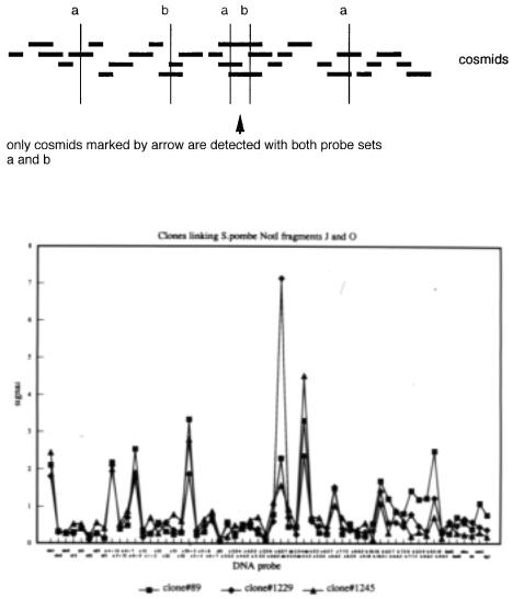
up clones with similar hybridization |
profiles |
that indicate possible overlaps (Box 8.3). |
The basic logic behind this method is shown in Figure 9.17. Regardless of how pools of probes are made, actually overlapping clones will tend to show a concordant pattern of hybridization when many probe pools are examined. The likelihoods that reflect the concordancy of the patterns were then used in a series of different clone-ordering algorithms, including those developed at LLNL, LANL, a cluster analysis, a simulated annealing
analysis, and the method sketched in Box 9.2. In general, we |
found |
that |
the different |
methods gave consistent results. Where inconsistencies were seen, |
these |
could |
often be |
resolved or rationalized by manual inspection of the data. Figure 9.18 shows the hybridization profile of three clones. This example was chosen because the interpretation of
the profile is straightforward. The clones share hybridization with the same chromosome, the same restriction fragments, and most of the same complex probe mixtures. Thus they
308 ENHANCED METHODS FOR PHYSICAL MAPPING
must |
be located |
nearby, |
and |
in fact they form a contig. The clones show some hybridiza- |
|
tion |
differences |
when |
very |
simple probe |
mixtures are used, since they are not identical |
clones. An example of the kinds of contigs that emerge from such an analysis is shown in |
|||||
Figure 9.19. These are clearly large |
and redundant contigs of the sort one hopes to see in |
||||
a robust map. |
|
|
|
|
|
Figure 9.17 |
Even when complex pools |
of probes are used (e.g., pools |
a and |
b ) overlapping clones |
will still tend to show a concordant pattern of |
hybridization. |
|
|
|
Figure |
9.18 |
Hybridization profile of three different |
S. pombe |
cosmid |
clones, |
with a series of 63 |
||
different pools of probes. |
|
|
|
|
|
|
||
|
|
|
|
|
|
|||
Figure 9.19 |
S. pombe |
cosmid map |
constructed from |
the patterns of probe hybridization to the |
S. |
|||
pombe |
cosmid |
array. Cosmids |
are indicated |
by horizontal |
lines along the maps. Letters shown |
|
|
|
above the map and fragment names (e.g., SHNF |
|
Sfi I fragment H and |
Not |
I fragment F). Gaps in |
||||
contigs are indicated by a vertical bar at the right end. Positions of LTRs, 5S rDNAs, and markers |
|
|
||||||
are indicated by *, #, and |
, respectively. |
|
|
|
|
|||

FALSE POSITIVES WITH SIMPLE POOLING SCHEMES |
309 |

310 ENHANCED METHODS FOR PHYSICAL MAPPING
BOX 9.2
CONSTRUCTION OF AN ORDERED CLONE MAP
Once a set of likelihood estimates has been obtained for clone overlap, the goal is to assemble a map of these clones that represents the most probable order given the available overlap data. This is a computationally intensive task. A number of different algorithms have been developed for the purpose. They all examine the consistency of particular clone orders with the likelihood results. The available methods all appear to be less than perfectly rigorous, since they all deal with data only on clone pairs and not on higher clusters. Nevertheless, these methods are fairly successful at establishing good ordered clone maps.
Figure 9.20 shows the principle behind a method we used in the construction of a
cosmid |
map of |
S. pombe. |
The objective in this limited example is to test the evidence |
|
in favor of particular schemes for ordering three clones A, B, and C. Various possible |
||||
arrangements of these clone are written as the columns and rows of a matrix, each ele- |
||||
ment of this matrix is represented by the maximum likelihood estimate that the clones |
||||
i and |
j overlap by a fraction |
f: L ij( f ). For each possible arrangement of clones, we cal- |
||
culated the weight of the matrix, |
W |
m defined as |
||
|
|
|
W m |
i j L ij(f) |
|
|
|
|
j i i |
The |
result for a simple case is shown in the figure. The true map will have an arrange- |
ment of clones that gives a minimum weight or very close to this. The method is par- |
|
ticularly effective in penalizing arrangements of clones where good evidence for over- |
|
lap |
exists, and yet the clones are postulated to be nonoverlapping in the final |
assembled map.
Figure 9.20 Example of an algorithm used to construct ordered clone maps from likelihood data. Details are given in Box 9.2.

|
FALSE |
POSITIVES WITH |
SIMPLE |
POOLING SCHEMES |
311 |
|||
The methods developed on |
S. pombe |
allowed a cosmid |
map |
to be completed to about |
|
|||
the 98% stage in 1.5 person years of effort. Most of this effort was method or algorithm |
|
|||||||
development, and we estimate that to repeat this process on a similar size genome would |
|
|
||||||
take only 3 person-months of effort. This is in stark contrast with earlier mapping ap- |
|
|||||||
proaches. Strict bottom-up fingerprinting methods, scaled to the size |
of |
the |
|
S. |
pombe |
|||
genome, would require around 8 to 10 person-years of effort. Thus by the use of pooling |
|
|
||||||
and complex probes, we have gained more than an order of magnitude in mapping speed. |
|
|
|
|||||
The issue that remains to be tested is how well this kind of approach will do with mam- |
|
|
||||||
malian samples where the effects of repeated DNA sequences will have to be eliminated. |
|
|
||||||
However, between the use of competition hybridization, which has been so successful in |
|
|
||||||
FISH, and selective PCR, we can be reasonably optimistic that probe pooling will be a |
|
|||||||
generally applicable method. |
|
|
|
|
|
|
|
|
FALSE POSITIVES WITH SIMPLE POOLING SCHEMES |
|
|
|
|
|
|
||
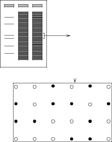
Row and column pools are very natural ideas for speeding the analysis |
of |
an |
array of |
|
|
|||
samples. It is easy to implement these |
kinds of pools with simple |
tools |
and |
robots. |
|
|||
However, they lead to a significant level of false positives when the density of positive |
|
|
||||||
samples in an array becomes large. Here |
we illustrate this problem in |
detail, |
since |
it |
|
|||
will be an even more serious problem in more complex pooling schemes. Consider the |
|
|
||||||
simple example shown in Figure 9.21. |
Here two clones in the array |
hybridize with |
a |
|
||||
probe (or show PCR amplification with the probe primers, in the case of YAC screening). |
|
|
||||||
If row and column pools are used for the analysis, rather than individual clones, four po- |
|
|
||||||
tentially positive clones are identified by the combination of two positive rows and two |
|
|
||||||
positive columns. Two are true positives; two are false positives. To decide among them, |
|
|
||||||
each isolated clone can be checked individually. In the case shown, only four additional |
|
|
||||||
hybridizations or PCR reactions would have to be done. This is a small addition to the |
|
|||||||
number of tests required for screening the rows and columns. However, as the number of |
|
|
||||||
true positives grows linearly, the number of false positives grows quadratically. It soon |
|
|
||||||
becomes hopelessly inefficient to screen them all individually. An alternative approach, |
|
|
||||||
which is much more efficient, in the limit of high numbers of positive samples, is to con- |
|
|
||||||
struct alternate pools. For example, in the case shown in Figure 9.21, if one also included |
|
|||||||
pools made along the diagonals, most true and false positives could be distinguished. |
|
|
|
|||||
Figure 9.21 An example of how false positives are generated when a pooled array is probed. Here row and sample pooling will reveal four apparent positive clones whenever only two real positives
occur (unless the two true positives happen to fall on the same row or column).
312 |
|
ENHANCED METHODS FOR PHYSICAL MAPPING |
|
|
||||
MORE |
GENERAL POOLING |
SCHEMES |
|
|
|
|
||
A |
branch |
of mathematics |
called |
sampling |
theory |
is |
well developed and instructs us how |
|
to |
design |
pools effectively. In the most |
general case there |
are two |
significant |
variables: |
||
the |
number |
of dimensions used for the array and the pools, |
and the number of alternate |
|||||
pool configurations employed. In the case described in Figure 9.21, the array is two di- |
||||||||
mensional, and the pools are one dimensional. Rows and columns represent one configu- |
||||||||
ration of the array. Diagonals, in essence, represent another configuration of the array be- |
||||||||
cause |
they |
would be rows and columns if the elements of |
the array were placed in a |
|||||
different order. Here we want to generalize these ideas. It is most important to realize that |
||||||||
the |
dimensionality of an |
array or a pool |
is a mathematical statement about how we |
chose |
||||
to describe it. It is not a statement about how the |
array is actually composed in space. An |
||
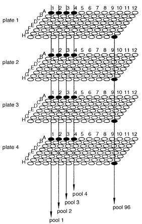
example is shown by the pooling scheme illustrated |
in Figure 9.22. Here plate pools are |
||
used in conjunction with vertical pools, made by combining each sample at a |
fixed |
x-ylo- |
|
cation on all the plates. The arrangement of plates appears to be three |
dimensional; |
the |
|
plate pools are two dimensional, but the vertical pools are only one dimensional. |
|
||
Figure 9.22 A pooling scheme that appears, superficially, to be three dimensional, but, in practice, is only two dimensional.
|
|
|
|
|
|
|
|
|
|
|
|
|
|
MORE GENERAL POOLING SCHEMES |
313 |
|||||||||||||
|
We |
consider |
first |
an |
N |
element library, |
and |
assume that we |
have |
sufficient |
robotics to |
|
|
|
|
|||||||||||||
sample it in any way we wish. A two-dimensional square array is constructed by assign- |
|
|
|
|
|
|
|
|
|
|||||||||||||||||||
ing to each element a location: |
|
|
|
|
|
|
|
|
|
|
|
|
|
|
|
|
|
|
|
|
|
|
|
|
||||
|
|
|
|
|
|
a ij |
|
where |
i 1, N |
1/2;j 1, N 1/2 |
|
|
|
|
|
|||||||||||||
If we pool rows and columns, each of these one-dimensional pools has |
|
|
|
|
|
|
|
|
|
|
|
|
N 1/2 components, |
|||||||||||||||
and |
there are 2 |
|
N 1/2 different |
pools if we |
just consider rows and columns. The |
|
actual |
con- |
|
|
|
|
|
|||||||||||||||
struction of a pool consists of setting one index constant, say |
|
|
|
|
|
|
|
|
|
|
i 3, and |
then |
combining |
|||||||||||||||
all samples that share that index. |
|
|
|
|
|
|
|
|
|
|
|
|
|
|
|
|
|
|
|
|
|
|
|
|||||
|
The |
same |
N |
element |
library |
can |
be treated |
as a |
three-dimensional |
cubic |
array. This is |
|
|
|
|
|
||||||||||||
constructed, by analogy, with the two-dimensional array by assigning to each element a |
|
|
|
|
|
|
|
|
|
|||||||||||||||||||
location: |
|
|
|
|
|
|
|
|
|
|
|
|
|
|
|
|
|
|
|
|
|
|
|
|
|
|
||
|
|
|
|
|
a ijk |
|
where |
|
|
i |
1, N |
1/3 |
|
|
1, N |
1/3 |
1, N |
1/3 |
|
|
|
|||||||
|
|
|
|
|
|
|
|
;j |
|
|
;k |
|
|
|
|
|
||||||||||||
If we pool two-dimensional surfaces of this array, each of these pools has |
|
|
|
|
|
|
|
|
|
|
|
N 2/3 compo- |
||||||||||||||||
nents. There are |
3 |
N 1/3 different |
pools if |
we |
consider |
|
three |
orthogonal sets |
|
of |
planes. The |
|
|
|
|
|||||||||||||
actual |
process of constructing |
these |
pools |
consists |
of |
setting |
one |
index |
constant, |
say |
|
|
|
|
|
|
||||||||||||
j 2, and then combining all samples that share this index. |
|
|
|
|
|
|
|
|
|
|
|
|
|
|
|
|
|
|||||||||||
|
We can easily generalize the pooling |
scheme |
to higher dimensions. These become |
|
|
|
|
|
|
|
||||||||||||||||||
hard |
to |
depict |
visually, but there is no |
difficulty |
at |
handling |
them |
mathematically. |
|
To |
|
|
|
|
|
|
|
|||||||||||
make a four-dimensional array of the library, we assign each of the |
|
|
|
|
|
|
|
|
|
|
|
N |
clones an index: |
|||||||||||||||
|
|
|
|
a ijkl |
where |
i |
1, N |
1/4 |
1, N |
1/4 |
|
|
|
1, N |
1/4 |
|
1, N |
1/4 |
|
|||||||||
|
|
|
|
|
;j |
|
;k |
|
;l |
|
|
|||||||||||||||||
This array is what is actually called a hypercube. |
We |
can |
make |
cubic |
pools |
of |
samples |
|
|
|
|
|
|
|
||||||||||||||
from the array by setting one index constant, say |
|
|
|
|
|
|
|
|
|
k |
4, |
and then combining all samples |
||||||||||||||||
that share this index. The result is 4 |
|
|
|
|
N |
1/4 different |
pools, |
each |
with |
|
|
|
N |
3/4 elements. The |
||||||||||||||
pools actually correspond to four orthogonal sets of sample cubes. |
|
|
|
|
|
|
|
|
|
|
|
|
|
|
|
|
||||||||||||
|
The process can be extended to five and higher dimensions as needed. Note that the re- |
|
|
|
|
|
|
|
|
|
||||||||||||||||||
sult of increasing the dimensionality is to decrease, steadily, the number of different pools |
|
|
|
|
|
|
|
|||||||||||||||||||||
needed, at a cost of increasing the size of each pool. Therefore the usefulness of higher- |
|
|
|
|
|
|
|
|||||||||||||||||||||
dimension pooling will depend very much on experimental sensitivity. Can the true posi- |
|
|
|
|
|
|
|
|
|
|||||||||||||||||||
tives b distinguished among an increasingly higher level of background noise as the com- |
|
|
|
|
|
|
|
|
|
|||||||||||||||||||
plexity of the pools grows? |
|
|
|
|
|
|
|
|
|
|
|
|
|
|
|
|
|
|
|
|
|
|
|
|
||||
|
The highest dimension possible for a pooling scheme is called a binary sieve. It is defi- |
|
|
|
|
|
|
|
||||||||||||||||||||
nitely the most efficient way to find a rare event in a complex sample so long as one is |
|
|
|
|
|
|
|
|||||||||||||||||||||
dealing with perfect data. In the examples discussed |
above, |
note that |
the |
range |
over |
|
|
|
|
|
|
|||||||||||||||||
which each sample index runs keeps dropping steadily, from |
|
|
|
|
|
|
|
|
|
|
|
i 1, |
N |
1/2 to |
i 1, N 1/4 as |
|||||||||||||
the dimension of the array is increased from two to four. The most extreme case possible |
|
|
|
|
|
|
|
|
|
|||||||||||||||||||
would allow each index only a single value; in this case there is really no array, the sam- |
|
|
|
|
|
|
|
|||||||||||||||||||||
ples are just being numbered. A pooling scheme one |
step short of this extreme would be |
|
|
|
|
|
|
|
|
|
||||||||||||||||||
to allow each index to run over just two numbers. If we kept strictly to the above analogy |
|
|
|
|
|
|
|
|||||||||||||||||||||
we would say |
|
i 1, 2; however, it is more useful to let the indices run from 0 to 1. Then |
|
|
|
|
||||||||||||||||||||||
we assign to a particular clone an index like |
|
|
|
|
|
|
|
a 101100. This is |
just a |
binary |
number |
(the |
||||||||||||||||
equivalent decimal is 44 in this case). Pools are constructed, just as |
before, |
by |
selecting |
|
|
|
|
|
||||||||||||||||||||
all clones with a fixed index, like |
|
|
a ijk 0mn . |
|
|
|
|
|
|
|
|
|
|
|
|
|
|
|
|
|||||||||
314 ENHANCED METHODS FOR PHYSICAL MAPPING
With a binary sieve we are nominally restricted to libraries where N 2 q. Then the array is constructed by indexing
N is a power of 2:
|
|
|
a ijklmn |
. . . |
|
|
where |
|
i, j, k, l, m,. n,. . 0, 1 |
|
|
|
|
|
|
|
|
|
|
|||||||||||
Each of the pools made by setting one index to a fixed value will have |
|
|
|
|
|
|
|
N |
/2 elements. The |
|
|
|||||||||||||||||||
number |
of |
pools will |
be |
|
q log( |
N |
)/log(2). This |
implicitly |
assumes that one scores each |
|
|
|
|
|
|
|
|
|
|
|||||||||||
clone for 1 or 0 at each index, but not both. The notion in a pure binary sieve is that if the |
|
|
|
|
|
|
|
|
|
|
|
|
||||||||||||||||||
clone |
is |
not in one pool (k |
|
|
1), |
it must certainly be in the other |
( |
|
k |
0), |
and so |
there |
is |
|
|
|||||||||||||||
no need to test them both. With real samples, one would almost certainly want to test both |
|
|
|
|
|
|
|
|
|
|
|
|
|
|||||||||||||||||
pools to avoid what are usually rather frequent false negatives. The size of each pool is |
|
|
|
|
|
|
|
|
|
|
|
|
||||||||||||||||||
enormous—it contains half of the clones in the library. However, the number of pools is |
|
|
|
|
|
|
|
|
|
|
|
|
|
|||||||||||||||||
very small. It cannot be further reduced without including additional sorts of information |
|
|
|
|
|
|
|
|
|
|
|
|
|
|||||||||||||||||
about the samples, such as intensity, color, or other measurable characteristics. |
|
|
|
|
|
|
|
|
|
|
|
|
|
|
|
|||||||||||||||
The |
binary sieve is constructed by numbering |
the |
samples |
with |
binary |
numbers, |
|
|
|
|
|
|
|
|
|
|
|
|
||||||||||||
namely integers in base two. One can back off from the extreme example of the binary |
|
|
|
|
|
|
|
|
|
|
|
|
|
|||||||||||||||||
sieve by using indices in other bases. For example, with base three indices, the array is |
|
|
|
|
|
|
|
|
|
|
|
|
||||||||||||||||||
constructed as |
a ijkl . . |
. , |
where |
|
i, j, k,.l,. |
. 0, 1, |
2. This results in a larger number of |
|
|
|
|
|
|
|||||||||||||||||
pools, each less complex than the pools used in the binary sieve. It is clear that to con- |
|
|
|
|
|
|
|
|
|
|
|
|
||||||||||||||||||
struct the actual pools used in binary sieves and related schemes would be |
quite complex |
|
|
|
|
|
|
|
|
|
|
|
|
|
||||||||||||||||
if one had to do it by hand. However, it is relatively easy to instruct an |
|
|
|
|
|
|
x-yrobot to sample |
|
|
|||||||||||||||||||||
in the required manner. Specialized tools could probably be utilized to make the pooling |
|
|
|
|
|
|
|
|
|
|
|
|
||||||||||||||||||
process more rapid. |
|
|
|
|
|
|
|
|
|
|
|
|
|
|
|
|
|
|
|
|
|
|
|
|
|
|
|
|
||
A numerical example will be helpful, here. Consider a library where |
|
|
|
|
|
|
|
|
N 2 14 16,384 |
|||||||||||||||||||||
clones. For a two-dimensional array, we need 2 |
|
|
|
|
|
|
|
7 by 2 |
7 or 128 by 128 clones. The row and |
|
|
|
|
|
|
|||||||||||||||
column pools will have 128 elements each. There are 256 pools needed. In contrast, the |
|
|
|
|
|
|
|
|
|
|
|
|
||||||||||||||||||
binary array requires only 14 pools (28 if we |
want to protect against false |
negatives). |
|
|
|
|
|
|
|
|
|
|
|
|
||||||||||||||||
Each pool, however, will have 8192 clones in it! Constructing these pools is not conceiv- |
|
|
|
|
|
|
|
|
|
|
|
|
||||||||||||||||||
able unless the procedure is fully automated. |
|
|
|
|
|
|
|
|
|
|
|
|
|
|
|
|
|
|
|
|
|
|
|
|
||||||
As the dimensionality of pooling increases, there are trade-offs between the reduced |
|
|
|
|
|
|
|
|
|
|
|
|
||||||||||||||||||
number |
of |
pools and the increased complexity of the |
pools. The advantage of reduced |
|
|
|
|
|
|
|
|
|
|
|
|
|
||||||||||||||
pool number is obvious: Fewer PCR reactions or hybridizations will have to be done. A |
|
|
|
|
|
|
|
|
|
|
|
|
||||||||||||||||||
disadvantage of increased pool complexity, beyond background problems that we have al- |
|
|
|
|
|
|
|
|
|
|
|
|
|
|
||||||||||||||||
ready discussed, is the increasing number of false positives when the array has |
a |
high |
|
|
|
|
|
|
|
|
|
|
|
|
||||||||||||||||
density of positive targets. For example, with |
|
a two-dimensional array, two |
positive |
|
|
|
|
|
|
|
|
|
|
|
|
|||||||||||||||
clones a |
36and a |
24 imply that false positives will appear at a |
|
|
|
|
34 and a |
26. In three dimensions, |
|
|
|
|||||||||||||||||||
two positive clones a |
|
826 |
and |
a |
534 |
will |
generate |
false |
positives |
at |
a |
|
824 |
, a |
|
, |
a |
834 |
, |
a |
|
, a |
524 |
, |
||||||
|
|
|
|
|
|
|
|
|
|
|
|
|
|
|
|
|
|
836 |
|
|
|
536 |
|
|||||||
and a |
|
. The number of false positives is smaller |
if |
some |
share |
a |
common |
orthogonal |
|
|
|
|
|
|
|
|
|
|
|
|
||||||||||
|
526 |
|
|
|
|
|
|
|
|
|
|
|
|
|
|
|
n |
|
|
|
|
|
|
|
|
|
|
|
|
|
plane. In |
general for |
two positive clones |
there will |
be |
up |
to 2 |
|
|
|
|
|
|
2 |
false |
positives |
in |
|
an |
|
|
|
|||||||||
n -dimensional pool. By the time a binary sieve is reached, the false positives become to- |
|
|
|
|
|
|
|
|
|
|
|
|
||||||||||||||||||
tally impossible to handle. Thus the binary sieve will be useful only for finding very rare |
|
|
|
|
|
|
|
|
|
|
|
|
||||||||||||||||||
needles in very large haystacks. For realistic screening of libraries, much lower dimen- |
|
|
|
|
|
|
|
|
|
|
|
|
||||||||||||||||||
sionality pooling is needed. |
|
|
|
|
|
|
|
|
|
|
|
|
|
|
|
|
|
|
|
|
|
|
|
|
|
|
|
|||
The actual optimum dimension pooling scheme to use will depend on the number of |
|
|
|
|
|
|
|
|
|
|
|
|
|
|||||||||||||||||
clones in the array, the redundancy of the library (which will increase the rate of false |
|
|
|
|
|
|
|
|
|
|
|
|
||||||||||||||||||
positives) and the number of false positives that one is willing to tolerate, and |
then |
re- |
|
|
|
|
|
|
|
|
|
|
|
|
||||||||||||||||
screen |
for individually or with |
an alternate array |
configuration. Figure |
9.23 |
gives |
some |
|
|
|
|
|
|
|
|
|
|
|
|
||||||||||||