Добавил:
Опубликованный материал нарушает ваши авторские права? Сообщите нам.
Вуз: Предмет: Файл:

Microcontroller based applied digital control (D. Ibrahim, 2006)

.pdf
Скачиваний:
1656
Добавлен:
12.08.2013
Размер:
5.68 Mб
Скачать

288 APPENDIX B MATLAB TUTORIAL

Arithmetic operators. MATLAB utilizes the following arithmetic operators:

+addition

-subtraction

*multiplication

/division

power operator

transpose

If x is a vector, its multiplication with a scalar multiplies all elements of the vector. For example,

>>x = [1, 3, 5];

>>y = 2*x

y =

2 6 10

Similarly, if A is a matrix, its multiplication with a scalar multiplies all elements of the matrix:

>> A =

[1 3; 5 7];

>> B =

2*A

B =


2

6

10

14

Two matrices can be multiplied to produce another matrix. For example, if


A =


2

4


and B =


5

2


1

3


2

4


then


>> A =

[1

3;

2

4];


>> B =

[2

4;

5

2];


>> C =

A B


C =


17

10


24

16


Array operations perform arithmetic operations in an element-by-element manner. An array operation is indicated by proceeding the operator by a period (.). For example, if a = [1 3 4] and b = [2 3 5] then

>>a = [1 3 4];

>>b = [2 3 5];

>>c = a.*b

c =

2 9 20

MATLAB OPERATIONS

289

Predefined functions. There are a number of predefined functions that can be used in statements. Some commonly used functions are:

abs

absolute value

sqrt

square root

real

real part

imag

imaginary part

rem

remainder

sin

sine

cos

cosine

asin

arcsine

acos

arccosine

tan

tangent

atan

arctangent

exp

exponential base e

log

natural logarithm

log10

log base 10

For example,

>>a = sqrt(16) a = 4

>>a = sqrt(-4) a = 0 + 2.0000i

Polynomials. A polynomial is defined by using a vector containing the coefficients of the polynomial. For example, the polynomial

F(x) = 3x4 5x3 + x2 3x + 1

is defined as

p = [3 -5 1 -3 1].

It is important that all powers of the polynomial must be specified. The coefficients of the missing powers must be specified as zero.

The following operations can be performed on a polynomial:

roots(p)

find the roots of the polynomial

polyval(p,x)

evaluate the polynomial p at the value of x

deconv(p1,p2)

compute the quotient of p1 divided by p2

conv(p1,p2)

compute the product of polynomials p1 and p2

poly(r)

compute the polynomial from the vector of roots

poly2str(p,‘s’)

display the polynomial as an equation in s

For example, consider the polynomial P1, where,

P1 = 6x4 2x3 + 5x2 2x + 1.

290 APPENDIX B MATLAB TUTORIAL

The roots of P1 = 0 are found as follows:

>>

P1 = [6 -2 5 -2 1]’

>>

r = roots(P1)

r =

-0.1026 + 0.8355i -0.1026 - 0.8355i 0.2692 + 0.4034i 0.2692 - 0.4034i

The polynomial has four complex roots.

The value of the polynomial at x = 1.2 is 14.7856 and can be found as follows:

>> polyval(P1, 1.2)

ans =

14.7856

The polynomial P1 can be expressed as an equation in s as:

>> poly2str(P1,‘s’)

ans =

6 s 4 - 2 s 3 + 5s 2 - 2 s + 1

Now consider another polynomial

P2 = 2x4 x3 + 2x2 x + 3.

The product of the polynomials P1 and P2 can be found as follows:

>> P2 =

[2 -1 2 -1

3];

>> P3

= conv(P1,P2)


P3 =


12

-10 24 -19

34 -16 19 -7 3

or


>> P3

=

poly2str(conv(P1,P2),‘x’)

P3 =

12x 8 - 10 x 7 + 24 x 6 - 19 x 5 + 34 x 4 - 16 x 3 + 19 x 2 - 7 x + 3

Finally, the polynomial whose roots are 2 and 5 can be found as follows:

>> poly([2 5])

ans =

1 -7 10
CONTROL SYSTEM TOOLBOX

291

or

>> poly2str(poly([2 5]),‘x’)

ans =

x 2 - 7x + 10

Thus, the equation of the required polynomial is

F(x) = x2 7x + 10.

B.2 CONTROL SYSTEM TOOLBOX

The Control System Toolbox is a collection of algorithms and uses MATLAB functions to provide specilized functions in control engineering. In this section we will briefly look at some of the important functions of the Control System Toolbox for both continuous-time and discrete-time systems.

B.2.1 Continuous-Time Systems

Consider a single-input, single-output continuous-time system with the open-loop transfer function

Y (s)

3


=


.

U (s)

s2 + 3s + 9

Transfer function. The transfer function of the system can be defined in terms of the numerator and the denominator polynomial:

>>num = [0 0 3];

>>den = [1 3 9];

The transfer function is given by:

>> G = tf(num,den)

Transfer function:

3

------------

s 2 + 3 s + 9

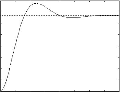
Step response. The step response is given by

>> step(num,den)

which produces the plot shown in Figure B.1.

292 APPENDIX B MATLAB TUTORIAL

Amplitude

Step Response

0.4

0.35

0.3

0.25

0.2

0.15

0.1

0.05

0

0

0.5

1

1.5

2

2.5

3

3.5

4

Time (sec)

Figure B.1 Step response

The steady-state value of the step response is obtained as follows:

>> ys = decgain(num,den)

ys =

0.3333

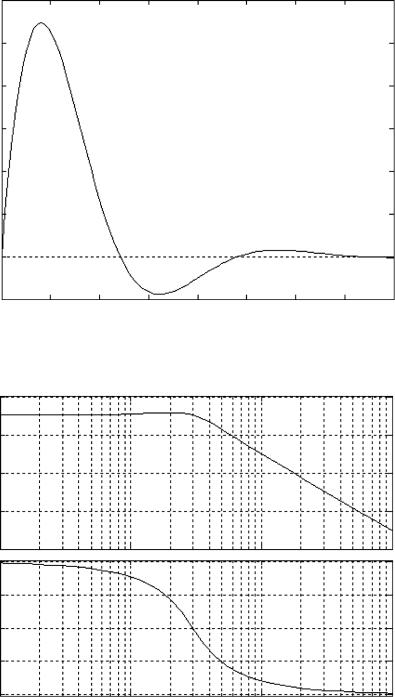
Impulse response. The impulse response is given by

>> impulse(num,den)

which produces the plot shown in Figure B.2.

Bode diagram. The Bode diagram can be obtained by writing:

>>impulse(num,den);

>>bode(num,den);

>>grid

Notice that the grid command produces a grid in the display. The Bode diagram of the system is shown in Figure B.3.

Nyquist diagram. The Nyquist diagram can be obtained from

>> nyquist(num,den)

The Nyquist diagram of the system is shown in Figure B.4.

CONTROL SYSTEM TOOLBOX

293


Impulse Response


0.6


0.5


0.4


Amplitude

0.3


0.2


0.1


0


0.1

0.5

1

1.5

2

2.5


0


Time (sec)


Figure B.2

Impulse response


Bode Diagram


0


(dB)

20


Magnitude

40


60


80


0


(deg)

45


90


Phase


135


180


10 1


100


101

Frequency (red/sec)

3

3.54

102

Figure B.3 Bode diagram

294 APPENDIX B MATLAB TUTORIAL

Imaginary Axis

Nyquist Diagram

1

0.8

0.6

0.4

0.2

0

0.2

0.4

0.6

0.8

11

0.8

0.6

0.4

0.2

0

0.2

0.4


Real Axis


Figure B.4 Nyquist diagram

Nichols diagram. The Nichols diagram can be obtained by writing

>>nichols(num,den);

>>grid

Figure B.5 shows the Nichols diagram obtained.

Root locus. The root locus diagram of the system is given by

>> rlocus(num,den)

Figure B.6 shows the graph obtained from this command.

To customize the plot for a specific range of K , say for K ranging from 0 to 5 in steps of 0.5, we can write

>>K = 0:0.5:5;

>>r = rlocus(num,den,K);

>>plot(r,‘x’)

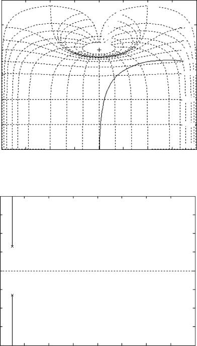
Figure B.7 shows the graph obtained, where the character x is plotted at the roots of the system as K is varied.

Zeros and poles. The zero and pole locations can be found from

>> [z,p,k] = tf2zp(num,den)

z =

Empty matrix: 0-by-1

Open-Loop Gain (dB)

Imaginary Axis

40

20

0

20

40

60

80 360

8

6

4

2

0

2

4

6

8

1.6


CONTROL SYSTEM TOOLBOX

295


Nichols chart


0 dB


0.25 dB


0.5 dB


1 dB


1 dB


3 dB


3 dB


6 dB


6 dB


12 dB


20 dB


40 dB


60 dB


80 dB

315

270

225

130

135

90

45

0


Open-Loop Phase (deg)


Figure B.5

Nichols diagram


Root Locus

1.4

1.2

1

0.8

0.6

0.4

0.2

0


Real Axis


Figure B.6 Root locus diagram

296

APPENDIX B MATLAB TUTORIAL


5


4


3


2


1


0


1


2


3


4


5

1.5 1.5 1.5

1.5

1.5 1.5 1.5 1.5


1.5

Figure B.7 Root locus diagram

p =

-1.5000 + 2.5981i -1.5000 - 2.5981i

k =

3

where z is the zeros, p is the poles and k is the gain.

Closed-loop system transfer function. The closed-loop system transfer function can be obtained using the feedback command. This command assumes by default a system a system with unity gain negative feedback. The closed-loop transfer function of the above system is thus given by

>>G = tf(num,den);

>>sys = feedback(G,1)

Transfer function:

3

-----------------

s^2 + 3s + 12

Series and parallel connected transfer functions. Consider two serially connected transfer functions G(s)H (s). The overall transfer function can be obtained as

series(G,H)

CONTROL SYSTEM TOOLBOX

297

where G and H are the transfer functions G(s) and H (s), respectively, in MATLAB representation. For example, if

1


2


G(s) =


and H (s) =


s2 + 3s + 4

s + 5

then G(s)H (s) can be obtained from


>>G = tf(1,[1 3 4]);

>>H = tf(2,[1 5]);

>>GH = series(G,H)

Transfer function:

2

--------------------------

s^3 + 8 s^2 + 19 s + 20

Similarly, the parallel statement can be used to reduce the transfer functions connected in parallel.

Factored transfer functions. If a transfer function is in factored form, it can be entered using the conv command. For example, if

G(s) =

(s + 4)

(s + 1)(s + 2)

then it can be entered into MATLAB as

>>num = [1 4];

>>den1 = [1 1];

>>den2 = [1 2];

>>den = conv(den1,den2);

Similarly, for the transfer function

G(s) =

2

(s + 1)(s + 2)(s + 4)

we can write

>>num = 2;

>>den1 = [1 1];

>>den2 = [1 2];

>>den3 = [1 4];

>>den = conv(den1,conv(den2,den3));

Inverse Laplace transforms. The MATLAB command residue is used to obtain the inverse Laplace transform of a transfer function by finding the coefficients of the partial fraction expansion. The partial fraction expansion is assumed to be in the following format:

Y (s) =


r(1)

+


r(2)

+


r(3)

+ · · · +


r(n)

+ k(s).

s

p(1)

s

p(2)

s

p(3)

s

p(n)