

Microcontroller based applied digital control (D. Ibrahim, 2006)
.pdf154 |
SAMPLED DATA SYSTEMS AND THE Z-TRANSFORM |
|
|||||||
|
e(s) |
|
e*(s) |
|
y(s) |
y*(s) |
|
||
|
G(s) |
|
|||||||
|
|
|
|
|
|
|
|
|
|
|
|
|
|
|
|
|
|
|
|
|
|
|
|
|
|
|
|
|
|
|
|
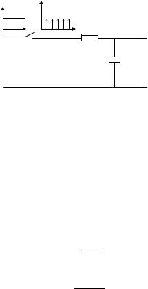
Figure 6.17 Sampling a system |
|
||||||
as illustrated in Figure 6.17. We sample the output signal to obtain |
|
||||||||
and |
y*(s) = [e*(s)G(s)]* = e*(s)G*(s) |
(6.34) |
|||||||
|
|
|
|
|
|
|
|
|
|
|
|
|
y(z) = e(z)G(z). |
|
|
(6.35) |
|||
Equations (6.34) and (6.35) tell us that if at least one of the continuous functions has been sampled, then the z-transform of the product is equal to the product of the z-transforms of each function (note that [e*(s)]* = [e*(s)], since sampling an already sampled signal has no further effect). G(z) is the transfer function between the sampled input and the output at the sampling instants and is called the pulse transfer function. Notice from (6.35) that we have no information about the output y(z) between the sampling instants.
6.3.1 Open-Loop Systems
Some examples of manipulating open-loop block diagrams are given in this section.
Example 6.15
Figure 6.18 shows an open-loop sampled data system. Derive an expression for the z-transform of the output of the system.
Solution
For this system we can write
y(s) = e*(s)KG(s)
or
y*(s) = [e*(s)KG(s)]* = e*(s)KG*(s)
and
y(z) = e(z)KG(z).
Example 6.16
Figure 6.19 shows an open-loop sampled data system. Derive an expression for the z-transform of the output of the system.
e(s) |
e*(s) |
|
y(s) |
y*(s) |
|||
G(s) |
|||||||
|
|
|
|
|
|
||
|
|
|
|
|
|
||
|
|
|
|
|
|
|
|
Figure 6.18 Open-loop system

PULSE TRANSFER FUNCTION AND MANIPULATION OF BLOCK DIAGRAMS |
155 |
||||||||
e(s) |
e*(s) |
|
|
|
|
y(s) |
y*(s) |
|
|
|
|
|
G1(s) |
|
|
G2(s) |
|
|
|
|
|
|
|
|
|
|
|
||
|
|
|
|
|
|
|
|
|
|
Figure 6.19 Open-loop system
Solution
The following expressions can be written for the system: y(s) = e*(s)G1(s)G2(s)
or
y*(s) = [e*(s)G1(s)G2(s)]* = e*(s)[G1G2]*(s)
and
y(z) = e(z)G1G2(z),
where
G1G2(z) = Z {G1(s)G2(s)} = G1(z)G2(z).
For example, if
G1(s) = 1 s
and |
|
|
|
|
|
|
|
|
|
|
|
|
|
|
|
|
|
|
|
|
|
|
|
G2(s) = |
|
a |
|
, |
|
|
|
|
|
|
|||
|
|
|
|
|
|
|
|
|
|
|
|
|
|
|
||||
|
|
|
|
|
s |
+ |
a |
|
|
|
|
|
||||||
then from the z-transform tables, |
|
|
|
|
|
|
|
|
|
|
|
|
|
|||||
|
|
|
|
|
|
|
|
|
|
|
|
|
|
|
||||
Z |
G |
(s)G |
(s) |
} = |
Z |
|
a |
|
|
|
= (z |
z(1 − e−aT ) |
||||||
|
|
a) |
|
|||||||||||||||
{ |
1 |
2 |
|
s(s |
+ |
− |
1)(z |
− |
e |
aT ) |
||||||||
|
|
|
|
|
|
|
|
|
|
|
|
|
|
|
− |
|||
and the output is given by
z(1 − e−aT )
y(z) = e(z) (z − 1)(z − e−aT ) .
Example 6.17
Figure 6.20 shows an open-loop sampled data system. Derive an expression for the z-transform of the output of the system.
e(s) |
e*(s) |
|
x(s) |
x*(s) |
|
y(s) |
y*(s) |
|||
G1(s) |
G2(s) |
|||||||||
|
|
|
|
|
|
|
|
|||
|
|
|
|
|
|
|
|
|||
|
|
|
|
|
|
|
|
|
|
|
Figure 6.20 Open-loop system

156 |
SAMPLED DATA SYSTEMS AND THE Z-TRANSFORM |
|
Solution |
|
|
The following expressions can be written for the system: |
|
|
or |
x(s) = e*(s)G1(s) |
|
|
|
|
and |
x*(s) = e*(s)G1*(s), |
(6.36) |
|
|
|
or |
y(s) = x*(s)G2(s) |
|
|
|
|
|
y*(s) = x*(s)G2*(s). |
(6.37) |
From (6.37) and (6.38),
y*(s) = e*(s)G*1 (s)G*2 (s),
which gives |
|
|
|
|
|
|
y(z) = e(z)G1(z)G2(z). |
|
|
|
|||
For example, if |
|
|
|
|
|
|
1 |
and G2(s) = |
|
a |
|
|
|
G1(s) = |
|
|
|
|
, |
|
s |
s |
+ |
a |
|||
|
|
|
|
|
|
|
then
Z {G1 |
(s)} = |
|
z |
|
|
and |
Z {G2(s)} = |
||||||||
z |
− |
1 |
|||||||||||||
and the output function is given by |
|
|
|
|
|
|
|
|
|
|
|
|
|||
|
|
|
|
|
|
|
|
|
|
|
|
|
|||
|
y(z) = e(z) |
|
z |
|
|
|
az |
||||||||
|
|
|
|
|
|||||||||||
or |
z − 1 |
z − ze−aT |
|||||||||||||
|
|
|
|
|
|
|
|
|
|
|
az |
|
|
||
|
y(z) = e(z) |
|
|
|
|
|
|
|
|||||||
|
|
|
|
|
|
||||||||||
|
(z |
− |
1)(1 |
− |
e aT ) |
||||||||||
|
|
|
|
|
|
|
|
|
|
|
|
− |
|||
az
z − ze−aT ,
.
6.3.2 Open-Loop Time Response
The open-loop time response of a sampled data system can be obtained by finding the inverse z-transform of the output function. Some examples are given below.
Example 6.18
A unit step signal is applied to the electrical RC system shown in Figure 6.21. Calculate and draw the output response of the system, assuming a sampling period of T = 1 s.
Solution
The transfer function of the RC system is
1
G(s) = . s + 1
PULSE TRANSFER FUNCTION AND MANIPULATION OF BLOCK DIAGRAMS |
157 |
R
u(s) |
u*(s) |
y(s) |
C
Figure 6.21 RC system with unit step input
For this system we can write
y(s) = u*(s)G(s)
and
y*(s) = u*(s)G*(s),
and taking z-transforms gives
y(z) = u(z)G(z).
The z-transform of a unit step function is
z
u(z) =
z − 1
and the z-transform of G(s) is
z
G(z) = z − e−T .
Thus, the output z-transform is given by
y(z) = u(z)G(z) = |
|
|
z |
|
|
|
z |
|
|
= |
|
|
z2 |
|
|
|
; |
|
z |
− |
1 z |
− |
e |
T |
(z |
− |
1)(z |
− |
e |
T ) |
|||||||
since T = 1 s and e−1 = 0.368, we get |
|
|
|
|
− |
|
|
|
|
− |
|
|
||||||
|
|
|
|
|
|
z2 |
|
|
|
|
|
|
|
|
|
|||
y(z) = |
|
|
|
|
|
|
|
|
. |
|
|
|
|
|
||||
(z |
− |
1)(z |
− |
0.368) |
|
|
|
|
|
|||||||||
|
|
|
|
|
|
|
|
|
|
|
|
|
|
|||||
The output response can be obtained by finding the inverse z-transform of y(z). Using partial fractions,
|
y(z) |
= |
|
|
A |
|
|
|
+ |
|
|
|
B |
|||
|
|
|
|
|
|
|
|
|
|
|
|
. |
||||
|
z |
z |
− |
|
1 |
|
z |
− |
0.368 |
|||||||
Calculating A and B, we find that |
|
|
|
|
|
|
|
|
|
|
|
|
|
|||
|
|
|
|
|
|
|
|
|
|
|
|
|
|
|
||
|
y(z) |
1.582 |
|
|
|
0.582 |
|
|
|
|||||||
|
|
|
|
|
|
|
|
|
|
|
|
|
|
|
|
|
|
z |
= z |
− |
1 |
− z |
− |
0.368 |
|||||||||
|
|
|
|
|||||||||||||
or |
|
|
|
|
|
|
|
|
|
|
|
|
|
|
|
|
y(z) = |
1.582z |
− |
|
0.582z |
||||||||||||
|
|
|
|
|
|
|
. |
|||||||||
z |
− |
1 |
|
z |
− |
0.368 |
||||||||||
|
|
|
|
|
|
|
|
|
|
|
|
|
|
|
||

158 SAMPLED DATA SYSTEMS AND THE Z-TRANSFORM
y(nT)
1.571
1.552
1.503
1.367
1.0
 T
T
0 |
T |
2T |
3T |
4T |
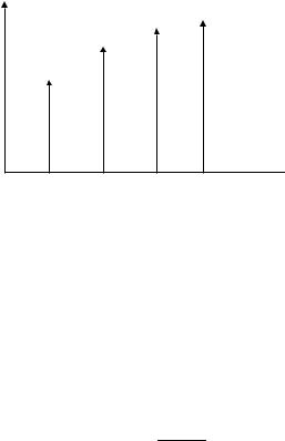
Figure 6.22 RC system output response
From the z-transform tables we find
y(nT ) = 1.582 − 0.582(0.368)n .
The first few output samples are
y(0) = 1,
y(1) = 1.367, y(2) = 1.503, y(3) = 1.552, y(4) = 1.571,
and the output response (shown in Figure 6.22) is given by
y(nT ) = δ(T ) + 1.367δ(t − T ) + 1.503δ(t − 2T ) + 1.552δ(t − 3T ) + 1.571δ(t − 4T ) + . . . .
It is important to notice that the response is only known at the sampling instants. For example, in Figure 6.22 the capacitor discharges through the resistor between the sampling instants, and this causes an exponential decay in the response between the sampling intervals. But this behaviour between the sampling instants cannot be determined by the z-transform method of analysis.
Example 6.19
Assume that the system in Example 6.17 is used with a zero-order hold (see Figure 6.23). What will the system output response be if (i) a unit step input is applied, and (ii) if a unit ramp input is applied.
|
|
|
G1(s) |
|
|
G2(s) |
|||||
u(s) |
u*(s) |
|
|
|
|
|
|
|
y(s) |
||
Z.O.H |
|
|
|
1 |
|
|
|||||
|
|
|
|
|
|
|
|
|
|||
|
|
|
|
|
|
s + 1 |
|
||||
|
|
|
|
|
|
|
|
|
|
|
|
Figure 6.23 RC system with a zero-order hold
PULSE TRANSFER FUNCTION AND MANIPULATION OF BLOCK DIAGRAMS |
159 |
Solution |
|
|
|
|
|
|
|
|
|
|
|
|
|
|
|
|
|
|
|
|
|
|
|
|
|
|
|
|
|
|
|
|
|
|
|
|
|
|
|
|
|
|
|
|
|
|
The transfer function of the zero-order hold is |
|
|
|
|
|
|
|
|
|
|
|
|
|
|
|
|
|
|
|
|
|
|
|
|
|
|
|
|
|
|
|
|
||||||||||||||
|
|
G |
1 |
(s) |
= |
1 − e−T s |
|
|
|
|
|
|
|
|
|
|
|
|
|
|
|
|
||||||||||||||||||||||||
|
|
|
|
|
|
|
|
|
|
|
|
|
|
|
|
|
|
|
|
|
|
|
|
|
|
|
|
|
|
|||||||||||||||||
|
|
|
|
|
|
|
|
|
|
|
|
|
|
|
|
s |
|
|
|
|
|
|
|
|
|
|
|
|
|
|
|
|
|
|
|
|
||||||||||
and that of the RC system is |
|
|
|
|
|
|
|
|
|
|
|
|
|
|
|
|
|
|
|
|
|
|
|
|
|
|
|
|
|
|
|
|
|
|
|
|
|
|
|
|
|
|
|
|
|
|
|
|
|
|
|
G(s) = |
|
|
|
1 |
|
|
|
|
|
. |
|
|
|
|
|
|
|
|
|
|
|
|
|
|
|
|
|
||||||||||||||
|
|
|
|
|
|
|
|
|
|
|
|
|
|
|
|
|
|
|
|
|
|
|
|
|
|
|
|
|
|
|
||||||||||||||||
|
|
|
|
|
s |
+ |
1 |
|
|
|
|
|
|
|
|
|
|
|
|
|
|
|
|
|
||||||||||||||||||||||
For this system we can write |
|
|
|
|
|
|
|
|
|
|
|
|
|
|
|
|
|
|
|
|
|
|
|
|
|
|
|
|
|
|
|
|
|
|
|
|
|
|
|
|
|
|
|
|||
|
|
|
|
|
|
|
|
|
|
|
|
|
|
|
|
|
|
|
|
|
|
|
|
|
|
|
|
|
|
|
|
|
|
|
|
|
|
|
|
|
|
|
|
|
||
|
|
y(s) = u*(s)G1G2(s) |
|
|
|
|
|
|
|
|
|
|
|
|
||||||||||||||||||||||||||||||||
and |
|
|
|
|
|
|
|
|
|
|
|
|
|
|
|
|
|
|
|
|
|
|
|
|
|
|
|
|
|
|
|
|
|
|
|
|
|
|
|
|
|
|
|
|
|
|
y*(s) = u*(s)[G1G2]*(s) |
|
|
|
|
|
|
||||||||||||||||||||||||||||||||||||||||
or, taking z-transforms, |
|
|
|
|
|
|
|
|
|
|
|
|
|
|
|
|
|
|
|
|
|
|
|
|
|
|
|
|
|
|
|
|
|
|
|
|
|
|
|
|
|
|
|
|
|
|
|
|
y(z) = u(z)G1G2(z). |
|
|
|
|
|
|
|
|
|
|
|
|
||||||||||||||||||||||||||||||||
Now, T = 1 s and |
|
|
|
|
|
|
|
|
|
|
|
|
1 − e−s |
|
|
|
|
1 |
|
|
|
|
|
|
|
|
|
|
|
|
||||||||||||||||
G |
G |
2 |
(s) |
= |
|
|
|
|
|
|
|
, |
|
|
|
|
|
|
|
|
||||||||||||||||||||||||||
|
|
|
|
|
|
|
|
|
|
s |
|
|
|
|
|
1 |
|
|
|
|
|
|
||||||||||||||||||||||||
1 |
|
|
|
|
|
|
|
|
|
|
|
s |
|
|
|
|
|
|
|
+ |
|
|
|
|
|
|
|
|
|
|
||||||||||||||||
and by partial fraction expansion we can write |
|
|
|
|
|
|
|
|
|
|
|
|
|
|
|
|
|
|
|
|
|
|
|
|
|
|
|
|||||||||||||||||||
|
|
|
|
|
|
|
|
|
|
|
|
|
|
|
|
|
|
|
|
|
|
|
|
|
|
|
|
|
|
|
|
|||||||||||||||
|
|
|
|
|
|
|
|
|
|
|
|
|
|
|
|
|
|
|
|
|
|
1 |
|
|
|
|
|
|
|
|
|
1 |
|
|
|
|
|
|
|
|
||||||
G1G2(s) = (1 − e−s ) |
|
|
|
|
|
− |
|
|
|
|
. |
|
|
|
||||||||||||||||||||||||||||||||
s |
|
|
s |
|
1 |
|
|
|
||||||||||||||||||||||||||||||||||||||
From the z-transform tables we then find that |
|
|
|
|
|
|
|
|
|
|
|
|
|
|
|
|
|
|
|
|
|
|
+ |
|
|
|
|
|
|
|
|
|||||||||||||||
|
|
|
|
|
|
|
|
|
|
|
|
|
|
|
|
|
|
|
|
|
|
|
|
|
|
|
|
|
|
|
|
|
||||||||||||||
G1G2(z) = (1 − z−1) |
|
|
|
|
|
z |
|
|
|
|
− |
|
|
|
|
|
|
z |
|
|
|
|
|
= |
|
0. |
63 |
. |
||||||||||||||||||
|
|
|
|
|
|
|
|
|
|
|
|
|
|
|
|
|||||||||||||||||||||||||||||||
z |
− |
1 |
z |
|
|
|
e |
− |
1 |
z |
− |
0.37 |
||||||||||||||||||||||||||||||||||
|
|
|
|
|
|
|
|
|
|
|
|
|
|
|
|
|
|
|
|
|
|
|
|
|
− |
|
|
|
|
|
|
|
|
|
|
|
|
|
|
|||||||
(i) For a unit step input, |
|
|
|
|
|
|
|
|
|
|
|
|
|
|
|
|
|
|
|
|
|
|
|
|
|
|
|
|
|
|
|
|
|
|
|
|
|
|
|
|
|
|
|
|
|
|
|
|
|
|
|
|
|
|
u(z) = |
|
|
|
z |
|
|
|
|
|
|
|
|
|
|
|
|
|
|
|
|
|
|
|
|
||||||||||||||
|
|
|
|
|
|
|
|
|
|
|
|
|
|
|
|
|
|
|
|
|
|
|
|
|
|
|
|
|
|
|
|
|
|
|||||||||||||
|
|
|
|
|
|
|
|
z |
− |
|
1 |
|
|
|
|
|
|
|
|
|
|
|
|
|
|
|
|
|
||||||||||||||||||
and the system output response is given by |
|
|
|
|
|
|
|
|
|
|
|
|
|
|
|
|
|
|
|
|
|
|
|
|
|
|||||||||||||||||||||
|
|
|
|
|
|
|
|
|
|
|
|
|
|
|
|
|
|
|
|
|
|
|
|
|
|
|
|
|
|
|
||||||||||||||||
|
y(z) = |
|
|
|
|
|
|
|
|
|
0.63z |
|
|
|
|
|
|
|
|
|
. |
|
|
|
|
|
||||||||||||||||||||
|
|
|
|
|
|
|
|
|
|
|
|
|
|
|
|
|
|
|
|
|
||||||||||||||||||||||||||
(z |
− |
1)(z |
− |
|
0.37) |
|
|
|
|
|
||||||||||||||||||||||||||||||||||||
|
|
|
|
|
|
|
|
|
|
|
|
|
|
|
|
|
|
|
|
|
|
|
|
|
|
|
|
|
|
|
|
|
|
|
|
|
|
|
|
|||||||
Using the partial fractions method, we can write |
|
|
|
|
|
|
|
|
|
|
|
|
|
|
|
|
|
|
|
|
||||||||||||||||||||||||||
|
y(z) |
|
|
|
= |
|
|
A |
|
|
|
|
|
+ |
|
|
|
|
|
|
|
B |
|
|
|
|
|
|
, |
|
|
|
|
|||||||||||||
|
|
|
|
|
|
|
|
|
|
|
|
|
|
|
|
|
|
|
|
|
|
|
|
|
|
|||||||||||||||||||||
|
|
z |
|
|
|
|
z |
− |
1 |
|
z |
− |
0.37 |
|
|
|
|
|
||||||||||||||||||||||||||||
where A = 1 and B = −1; thus, |
|
|
|
|
|
|
|
|
|
|
|
|
|
|
|
|
|
|
|
|
|
|
|
|
|
|
|
|
|
|
|
|
|
|
|
|
|
|
||||||||
|
|
|
|
|
|
|
|
|
|
|
z |
|
|
|
|
|
|
|
|
|
|
|
|
|
|
|
|
|
z |
|
|
|
|
|
|
|
|
|
|
|
|
|||||
|
y(z) = |
|
|
|
|
|
|
|
|
− |
|
|
|
|
|
|
|
|
|
|
|
|
. |
|
|
|
|
|
||||||||||||||||||
|
|
|
|
|
|
|
|
|
|
|
|
|
|
|
|
|
||||||||||||||||||||||||||||||
|
z |
− |
1 |
z |
|
− |
0.37 |
|
|
|
|
|
||||||||||||||||||||||||||||||||||
|
|
|
|
|
|
|
|
|
|
|
|
|
|
|
|
|
|
|
|
|
|
|
|
|
|
|
|
|
|
|
|
|
|
|
|
|
|
|
|
|
||||||
160 SAMPLED DATA SYSTEMS AND THE Z-TRANSFORM
y(nT)
0.98 0.95
0.86
0.63
 T
T
0 |
T |
2T |
3T |
4T |
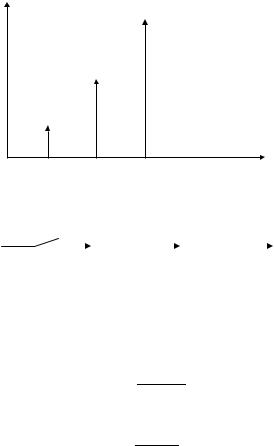
Figure 6.24 Step input time response of Example 6.19
From the inverse z-transform tables we find that the time response is given by
y(nT ) = a − (0.37)n ,
where a is the unit step function; thus
y(nT ) = 0.63δ(t − 1) + 0.86δ(t − 2) + 0.95δ(t − 3) + 0.98δ(t − 4) + . . . .
The time response in this case is shown in Figure 6.24.
(ii) For a unit ramp input,
u(z) =
T z
(z − 1)2
and the system output response (with T = 1) is given by
y(z) = |
0.63z |
= |
0.63z |
||
|
|
|
. |
||
(z − 1)2(z − 0.37) |
z3 − 2.37z2 + 1.74z − 0.37 |
||||
Using the long division method, we obtain the first few output samples as
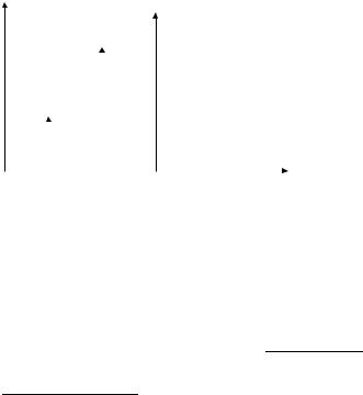
y(z) = 0.63z−2 + 1.5z−3 + 2.45z−4 + 3.43z−5 + . . .
and the output response is given as
y(nT ) = 0.63δ(t − 2) + 1.5δ(t − 3) + 2.45δ(t − 4) + 3.43δ(t − 5) + . . . ,
as shown in Figure 6.25.
Example 6.20
The open-loop block diagram of a system with a zero-order hold is shown in Figure 6.26. Calculate and plot the system response when a step input is applied to the system, assuming that T = 1 s.
PULSE TRANSFER FUNCTION AND MANIPULATION OF BLOCK DIAGRAMS |
161 |
y(nT)
2.45
1.5
0.63
T
2T |
3T |
4T |
Figure 6.25 Ramp input time response of Example 6.19
|
|
|
G1(s) |
|
|
|
G2(s) |
|
|
|
||
u(s) |
u*(s) |
|
|
|
|
|
|
|
|
|
||
Z.O.H |
|
|
|
1 |
|
|
y(s) |
|||||
|
|
|
|
|
|
|
|
|
|
|||
|
|
|
|
|
|
s(s + 1) |
|
|
|
|||
|
|
|
|
|
|
|
|
|
|
|
|
|
Figure 6.26 Open-loop system with zero-order hold
Solution
The transfer function of the zero-order hold is
G1(s) =
1 − e−T s
s
and that of the plant is
1
G(s) = . s(s + 1)
For this system we can write
y(s) = u*(s)G1G2(s)
and
y*(s) = u*(s)[G1G2]*(s)
or, taking z-transforms,
y(z) = u(z)G1G2(z).
Now, T = 1 s and |
|
|
|
1 − e−s |
|
|
|
|
|
||||||
G |
G |
(s) |
|
|
|
|
|
|
|||||||
|
|
|
|
|
|
|
|
|
|
|
|||||
1 |
2 |
|
= s2(s |
+ |
1) |
|
|
|
|
|
|||||
or, by partial fraction expansion, |
|
|
|
|
|
|
|
|
|
|
|
|
|
|
|
|
|
|
|
|
|
|
|
|
|
|
|
|
|
|
|
G1G2(s) = (1 − e−s ) |
1 |
|
|
1 |
|
|
|
1 |
|
|
|||||
|
− |
|
|
+ |
|
|
|||||||||
s2 |
s |
s |
+ |
1 |
|||||||||||
|
|
|
|
|
|
|
|
|
|
|
|
|
|
|
|
162 SAMPLED DATA SYSTEMS AND THE Z-TRANSFORM
y(nT)
0.9145
0.7675
|
|
|
|
|
|
|
0.3678 |
|
|
|
|
|
|
|
|
|
|
|
|
|
|
|
|
|
|
|
|
|
|
|
|
|
|
|
|
|
|
|
|
|
|
|
|
|
|
|
|
|
|
|
|
|
|
|
|
|
|
|
|
|
|
|
|
|
|
|
|
|
T |
|
|
|
|
|
|
|
|
|
|
|
|
|
|
|
|
|
|
|
|
|
|
|
|
|
|
|
|
|
|
|
|
|
|
|
|
|
|
|
|
|
|
|
|
|
0 |
|
T |
|
2T |
3T |
|
|
|
|
|
|
|
|
|
|
|
|
|
|
|
|
|
|
|
||||||||
|
|
|
|
|
|
|
|
|
|
|
|
|
|
|
|
|
|
|
|
|
|
|
|
|
|
|||||||||||
|
|
|
|
|
|
|
|
Figure 6.27 Output response |
|
|
|
|
|
|
|
|
|
|
|
|
||||||||||||||||
and the z-transform is given by |
|
|
|
|
|
|
|
|
− s |
|
+ s 1 |
|
1 . |
|
|
|
|
|
|
|
||||||||||||||||
|
|
|
|
|
|
G1G2(z) = (1 − z−1)Z s2 |
|
|
|
|
|
|
|
|
|
|||||||||||||||||||||
|
|
|
|
|
|
|
|
|
|
|
|
|
|
|
|
|
1 |
|
|
1 |
|
|
|
|
|
|
|
|
|
|
|
|
|
|
|
|
From the z-transform tables we obtain |
|
|
|
|
|
|
|
|
|
|
+ |
|
|
|
|
|
|
|
|
|
|
|||||||||||||||
|
|
|
|
|
|
|
|
|
|
|
|
|
|
|
|
|
|
|
|
|
|
|||||||||||||||
G |
G |
(z) |
|
(1 |
|
z−1) |
|
z |
|
|
|
|
z |
|
|
|
|
|
z |
|
|
|
|
|
|
ze−1 + 1 − 2e−1 |
||||||||||
= |
− |
|
|
1)2 − z |
|
1 |
+ z |
|
|
e |
|
1 |
= |
|
||||||||||||||||||||||
1 |
2 |
|
|
|
|
(z |
− |
− |
− |
− |
|
(z |
− |
1)(z |
− |
e |
− |
1) |
||||||||||||||||||
|
|
|
|
|
|
|
|
|
|
|
|
|
|
|
|
|
|
|
|
|
|
|
|
|
|
|
|
|||||||||
|
|
|
|
|
|
0.3678z + 0.2644 |
. |
|
|
|
|
|
|
|
|
|
|
|
|
|
|
|
|
|
|
|
|
|
|
|||||||
|
|
|
= z2 − 1.3678z + 0.3678 |
|
|
|
|
|
|
|
|
|
|
|
|
|
|
|
|
|
|
|
|
|
|
|||||||||||
After long division we obtain the time response
y(nT ) = 0.3678δ(t − 1) + 0.7675δ(t − 2) + 0.9145δ(t − 3) + . . . ,
shown in Figure 6.27.
6.3.3 Closed-Loop Systems
Some examples of manipulating the closed-loop system block diagrams are given in this section.
Example 6.21
The block diagram of a closed-loop sampled data system is shown in Figure 6.28. Derive an expression for the transfer function of the system.
Solution |
|
For the system in Figure 6.28 we can write |
|
e(s) = r(s) − H (s)y(s) |
(6.38) |
and |
|
y(s) = e*(s)G(s). |
(6.39) |
PULSE TRANSFER FUNCTION AND MANIPULATION OF BLOCK DIAGRAMS |
163 |
||||||||||
r(s) |
|
e(s) |
|
e*(s) |
|
|
y(s) |
|
|||
G(s) |
|
|
|||||||||
|
|
|
|
|
|
|
|
|
|||
|
|
|
|
|
|
|
|
|
|
||
|
+ − |
|
|
|
|
|
|
||||
|
|
|
|
|
|
|
|
|
|||
|
|
|
|
|
|
|
|
|
|||
|
|
|
|
|
|
|
|
|
|
|
|
|
|
|
|
H(s) |
|
|
|
|
|
|
|
|
|
|
|
|
|
|
|
|
|
|
|
Figure 6.28 Closed-loop sampled data system
Substituting (6.39) into (6.38),
e(s) = r(s) − G(s)H (s)e*(s)
or
e*(s) = r*(s) − GH*(s)e*(s) and, solving for e*(s), we obtain
e*(s) = |
|
r*(s) |
||||||||
1 + GH*(s) |
|
|
|
|||||||
and, from (6.39), |
|
|
|
|
|
|
|
|
||
y(s) = G(s) |
|
r*(s) |
||||||||
|
|
|
|
. |
||||||
1 + GH*(s) |
||||||||||
The sampled output is then |
|
|
|
|
|
|
|
|
||
y*(s) = |
r*(s)G*(s) |
|||||||||
1 + GH*(s) |
|
|||||||||
Writing (6.43) in z-transform format, |
|
|
|
|
|
|
|
|
||
|
y(z) = |
r(z)G(z) |
||||||||
|
|
|
|
|
|
|||||
1 |
+ |
GH(z) |
||||||||
and the transfer function is given by |
|
|
|
|
|
|
|
|||
|
|
|
|
|
|
|
|
|||
|
y(z) |
|
G(z) |
|||||||
|
|
= |
|
|
|
. |
||||
|
r(z) |
1 |
+ |
GH(z) |
||||||
|
|
|
|
|
|
|
|
|
|
|
Example 6.22
(6.40)
(6.41)
(6.42)
(6.43)
(6.44)
(6.45)
The block diagram of a closed-loop sampled data system is shown in Figure 6.29. Derive an expression for the output function of the system.
Solution |
|
For the system in Figure 6.29 we can write |
|
y(s) = e(s)G(s) |
(6.46) |