Microcontroller based applied digital control (D. Ibrahim, 2006)

124 MICROCONTROLLER PROJECT DEVELOPMENT

Sum Of

Numbers

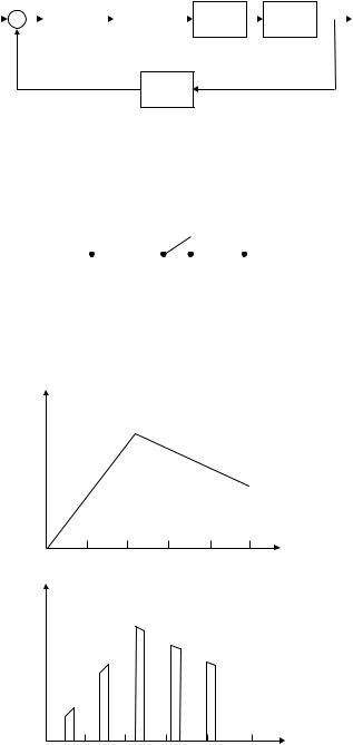
Figure 5.7 Structure chart for Example 5.1

of the details of the target language. There are no fixed rules or standards for developing pseudocode, and individual designers may have their own personal style of pseudocode. There are, however, guidelines to help the designer develop readable and powerful pseudocode. Pseudocode is based on the concept that any program consists of three major items: sequencing, selection, and iteration. Pseudocode is then developed using English sentences to describe algorithms, and this code cannot be compiled. If a program consists of a number of modules called by the main program then each module should be described using pseudocode. A brief description of the verbs and sentences that can be used in pseudocode is given in the rest of this section.

5.2.3.1 BEGIN–END

This construct is used to declare the beginning and end of a program or module. Keywords such as ‘:MAIN’ can be used before BEGIN to declare the beginning of the main program:

:MAIN BEGIN

. . .

. . .

END

Alternatively, the module name can be used:

:ADD BEGIN

. . .

. . .

END

As shown in these examples, the lines should be indented to make the algorithm easier to read.

5.2.3.2 Sequencing

A sequence is a linear progression where the tasks are performed sequentially one after the other. Each action should be written on a new line and all the actions should be aligned with the same indent. The following keywords can be used for the description of the algorithm:

For example:

:MAIN BEGIN

Read three numbers Calculate their sum Display the result

END

5.2.3.3 IF–THEN–ELSE–ENDIF

The keywords IF, THEN, ELSE and ENDIF can be used to indicate that a decision is to be made. The general format of this construct is:

IF condition THEN statement statement

ELSE statement statement

ENDIF

The ELSE keyword and the statements following it are optional. In the following example they are omitted:

IF grade > 90 THEN

Letter = ‘A’

ENDIF

If the condition is true, the statements following the THEN are executed, otherwise the statements following the ELSE are executed. For example:

IF temperature > 100 THEN

Turn off heater

Start the engine

126 MICROCONTROLLER PROJECT DEVELOPMENT

ELSE

Turn on heater

ENDIF

5.2.3.4 REPEAT–UNTIL

This construct is used to specify a loop where the test is performed at the end of the loop, i.e. the loop is executed at least once, perhaps many times, depending upon the condition at the end of the loop. The loop continues forever if the condition is not satisfied. The general format is:

REPEAT

Statement

Statement

Statement

UNTIL condition

In the following example the statements inside the loop are executed five times:

Set cnt = 0

REPEAT

Turn on LED

Wait 1 s

Turn off LED

Wait 1 s

Increment cnt

UNTIL cnt = 5

5.2.3.5 DO–WHILE

This construct is similar to REPEAT–UNTIL, but here the loop is executed while the condition is true. The condition is tested at the end of the loop. The general format is:

DO statement statement statement

WHILE condition

In the following example the statements inside the loop are executed five times:

Set cnt = 0

DO

Turn on LED

Wait 1 s

Turn off LED

Wait 1 s

Increment cnt

WHILE cnt < 5

5.2.3.6 WHILE–WEND

This construct is similar to REPEAT–UNTIL, but here the loop may never be executed, depending on the condition. The condition is tested at the beginning of the loop. The general format is:

WHILE condition statement statement statement

WEND

In the following example the loop is never executed:

I = 0

WHILE I > 0

Turn on LED

Wait 3 s

WEND

In this next example the loop is executed 10 times:

I = 0

WHILE I < 10

Turn on motor

Wait 2 seconds

Turn off motor

Increment I

WEND

5.2.3.7 CASE–CASE ELSE–ENDCASE

The CASE construct is used for multi-way branch operations. An expression is selected and, based on the value of this expression, a number of mutually exclusive tests can be done and statements can be executed for each case. The general format of this construct is:

CASE expression OF condition1:

statement statement condition2: statement statement condition3: statement statement

. . .

. . .

128 MICROCONTROLLER PROJECT DEVELOPMENT

CASE ELSE

Statement

Statement

END CASE

If the expression is equal to condition1, the statements following condition1 are executed, if the expression is equal to condition2, the statements following condition2 are executed and so on. If the expression is not equal to any of the specified conditions then the statements following the CASE ELSE are executed.

In the following example the points obtained by a student are calculated based on the grade:

CASE grade OF

A:points = 10

B:points = 8

C:points = 6

D:points = 4

CASE ELSE points = 0

END CASE

Notice that the above CASE construct can be implemented using the IF–THEN–ELSE construct as follows:

IF grade = A THEN points = 10

ELSE IF grade = B THEN points = 8

ELSE IF grade = C THEN points = 6

ELSE IF grade = D THEN points = 4

ELSE points = 0

END IF

5.2.3.8 Invoking Modules

Modules can be called using the CALL keyword and then specifying the name of the module. It is useful if the input parameters to be passed to the module are specified when a module is called. Similarly, at the header of the module description the input and the output parameters of a module should be specified. An example is given below.

Example 5.2

Write the pseudocode for an application where three numbers are read from the keyboard into a main program, their sum calculated using a module called SUM, and the result displayed by the main program.

Solution

The pseudocode for the main program and the module are given in Figure 5.8.

:MAIN BEGIN

Read 3 numbers a, b, c from the kayboard Call SUM (a, b, c)

Display result

END

:SUM (I: a, b, c O: sum of numbers) BEGIN

Calculate the sum of a, b, c Return sum of numbers

END

Figure 5.8 Pseudocode for Example 5.2

5.3 EXERCISE

1.What are the three major components of a flow chart? Explain the function of each component with an example.

2.Draw a flow chart for a simple sort algorithm.

3.Draw a flow chart for a binary search algorithm.

4.What are the differences between a flow chart and a structure chart?

5.What are the three major components of a structure chart? Explain the function of each component with an example.

6.Draw a flow chart to show how a quadratic equation can be solved.

7.What are the advantages of pseudocode?

8.What are the basic components of pseudocode?

9.Write pseudocode to read the base and the height of a triangle from the keyboard, call a module to calculate the area of the triangle and display the area in the main program.

10.Explain how iteration can be done in pseudocode. Give an example.

11.Give an example of pseudocode to show how multi-way selection can be done using the CASE construct. Write the equivalent IF–ELSE–ENDIF construct.

FURTHER READING

[Baker, and Scallon, 1986] Baker, T.P. and Scallon, G.M. An architecture for real-time software systems IEEE Trans. Software Mag., 3, 3, 1986, pp. 50–58.

6

Sampled Data Systems and the z-Transform

A sampled data system operates on discrete-time rather than continuous-time signals. A digital computer is used as the controller in such a system. A D/A converter is usually connected to the output of the computer to drive the plant. We will assume that all the signals enter and leave the computer at the same fixed times, known as the sampling times.

A typical sampled data control system is shown in Figure 6.1. The digital computer performs the controller or the compensation function within the system. The A/D converter converts the error signal, which is a continuous signal, into digital form so that it can be processed by the computer. At the computer output the D/A converter converts the digital output of the computer into a form which can be used to drive the plant.

6.1 THE SAMPLING PROCESS

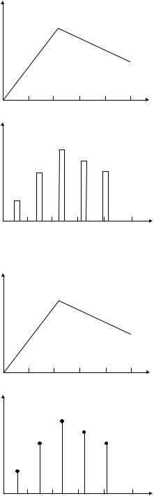
A sampler is basically a switch that closes every T seconds, as shown in Figure 6.2. When a continuous signal r(t) is sampled at regular intervals T , the resulting discrete-time signal is shown in Figure 6.3, where q represents the amount of time the switch is closed.

In practice the closure time q is much smaller than the sampling time T , and the pulses can be approximated by flat-topped rectangles as shown in Figure 6.4.

In control applications the switch closure time q is much smaller than the sampling time T and can be neglected. This leads to the ideal sampler with output as shown in Figure 6.5.

The ideal sampling process can be considered as the multiplication of a pulse train with a continuous signal, i.e.

Microcontroller Based Applied Digital Control D. Ibrahim

C 2006 John Wiley & Sons, Ltd. ISBN: 0-470-86335-8